• View
• Edit
• History
• Print

Muzen

< cctbx initial trial | Index | Hypothesis on an ideal molecular magnet >

Muzen

We shall briefly sketch the use of one analysis program (not because of its peculiar virtues).

A very general suggestion is to keep:

• a directory for each instrument, call it $gps, with a startup file MUZEN.DAT properly tuned for the instrument characteristics
• a directory (or a user) for raw data, with a standard structure, such as e.g. musr/psi/gps/run_10_05/mysample/; then Muzen can automatically replicate the same structure under a different root (e.g. gps)

The suggested strategy within this program is to fit asymmetries from pairs, or groups of detectors. This implies:

• choosing the appropriate grouping
• having one or more data sets with low transverse field to calibrate the parameter {$\alpha$}.

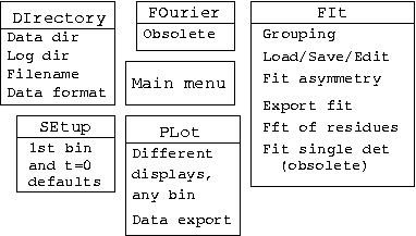
The program is console driven, under linux. The sketch on the right shows the main and the secondary menues, accessed by (case unsensitive) typing their first two letters (capitalized in the menu) and carriage return (CR). If the setup is correct for the instrument, most of the time is spent in menu FIt, where data loading, fit function selection, saving and reloading, fit execution, plotting, fft of residues and saving of results can be chosen by entering the unique initial of the each menu item.

The asymmetry fit function can be chosen adding a number of preset components among those available, described below and in the Relaxation function pages. The implementation of totally new fit functions is beyond the scope of this description.

Nearly complete list of menu keys:

• DIrectory
  • Current run on certain systems allows to read data from the data acquisition setup; nearly obsolete.
  • Directory where the data resides
  • Facility data formats
  • Logdir where the logs are written; the format is $dirname$n where dirname is the portion of the linux directory name, say /home/musr/psi/gps/run_10_05/mysample/ after which the name si replicated, starting from the directory where Muzen is launched from, e.g. /home/user/muzen/psi/gps/; in this example $gps$2 will place the logs in /home/user/muzen/psi/gps/run_10_05/mysample/, creating it if it does not exist.
  • Prefix data file name prefix, this and the following ar erules for renaming your data files; suggestion: gps, ltf, dol, mus, emu, etc.; the full name should be something like insxxxxx.suf with space for 5 unique digits (this does not compy with ISIS naming scheme any more, and will be updated)
  • Specification data file name suffix, it is data format specific: dat (ASCII psi), bin (new PSI), nxs (new ISIS), raw (old ISIS)

SEtup Offset defaults how many channels must be skipped from the first read in the analysis; e.g. if Offset=6 and Range=[1 5000] the first used bin is the sixth; at ISIS this means the sixth in the data set, while at PSI the first would be the first-good-bin recorded in the data header and selected from the acquisition program. Beam structure & prompt T0(ns)distance from the right time t=0 and the center of bin 1. Show offset and prompt ditto bacKground@psi the uncorrelated background at psi is automatically determined by the program at load time, by fitting the bin content for times t<0; the plot on the right illustrates these two integers.

First 300 bins from a typical GPS detector time-histogram: zero counts up to bin 50, uncorrelated background {$N_u$} up to bin 200, a prompt-particle centered peak at bin 209, and the positrons from muon decays from there on. Muzen evaluates {$N_u$} from the tip of the second horizontal arrow to the tip of the third, and bacKground requires how many bins to skip from the start of the uncorrelated background and how many before the prompt (the two intervals indicated by the horizontal arrows).

• WRite setup writes file MUZEN.DAT containing the DIrectory information, the SEtup incorfmation and a default grouping
• INput to load a file, please set the correct data format, directory and log directory first.
• PLot (|CR|), graphical displays;
  Offset is inactive in these subroutines and all loaded channels may be displayed (PSI data are loaded starting from first bin, as encoded in the file header);
  All display routines start with an infinite loop range request (always in bins, or channels), to exit enter range 0 0;
  graphics is handled by /Plplot, providing a Plplot> prompt for printing (to exit press Carriage Return (|CR|), for print options type H);
  • Alpha [1.0 ] see the FIt description
  • Bin [ 1} rebinning
  • For-or-back shows sum of all Forward or all Backwards detector counts in the present Grouping
  • Logarithmic plot of individual detectors, useful to check uncorrelated background levels
  • Normal plot of individual detector, the basic inspection tool,
  • Polarization yields asymmetry plot according to preset Grouping
  • Reset grouping to redefine the Grouping
  • Smartplot, (not so smart!) Polarization plot with automatic increment of binning, so as to keep data errorbar roughly constant with time.
  • Multiplot exports data in Polarization (asymmetry) format; creates file filename.x with one columns (time), appends data to file filename.y in successive columns (do not exceed four to avoid wrapping) and likewise errors to filename.e
  • Write smartplot exports in smartplot format
• SImulate data a stub
• FOurier transform obsolete (use FFT of residues instead)

• EXclude histo to temporarily Delete detectors from a large ISIS grouping or to Restore them (see note).
• SLow-mu in a stub
• QUit ditto
• FIt
  • if model does not exist yet:
    • Read input read model file from the $gps directory, where basic models may be stored with the following name scheme: aabbcc.fit is a three component model, where aa is the first two letters of the component name (suffix is default), e.g. bamumu.fit has a longitudinal relaxation BACK plus two transverse precessing components MU+.
    • Polarization chose asymmetry fit
      • How many components? answer e.g. 3 for two BACK and one MU+.

     1 -   DA: p=((2+DA/alpha)*p-DA/alpha)/ ((2+DA/alpha)-Da/alpha*p)
     2 - MU+.: A cos(2pi (gam_mu B t + PHI/360)) exp(-L t) exp(-(G t)^2/2)
     3 - BJ0+: A J0(2pi (gam_mu B t + PHI/360)) exp(-L t) exp(-(G t)^2/2)
     4 - BACK: A exp(-L t) exp(-(G t)^2/2)
     5 - K-T.: KTLo KTGa (DELO,DEGA) in B(GAU), dyn (wdyn),T1:exp(-L t)
     6 - PWKT: PowerKT: Alfa=static, Beta= dyn expo, GAU=B PRL72(1994)3722
     7 - PINK: Uemura - Pinkvos function: J. Physique C8(1988)1035
     8 - STEX: A cos(2 pi (gamma_mu B t + PHI/360)) exp(-(L t)^BETA)
     9 - MISC: Miscount correct:f=[(1+daa)eb-ef-daa]/[2+daa-ef-(1+daa)eb]
    10 - MUOT: Mu Triplet: Atot,n0=hyp freq,B(GAU),nu12-23 decay=DE+-dD
    11 - PWRD: New PowerKT: beta=dyn exp (alpha=2beta), a_s=static width
    12 - FMuF: Linear F-Mu-F model: 3 freq out of a dipolar field
    13 - KERN: Keren appro. dynam. K.-T.(PRB 50(14)10039)
    14 - FLL : Flux line lattice(pb.m) LMnm XInm lambda&xi(nm) DEGA broad

• Select from the above list use the numbers on the left of the given list

• Decay histo choose single detector fit (obsolete, not working properly)
• Global a few complex components for a fit involving four GPS detectors at once, implementing the general formula, including an external field (not documented yet)
• Quit ditto

• if model exists
  • Alpha [1.0 ] to change the displayed value of {$\alpha$} (Eq. 3), used for calculating the asymmetry. Typically use a fit model damu to determine the correct value on a low transverse field data set: starting with a rough estimate of Alpha, the fitted value of parameter DA must be subtracted from Alpha to get a better estimate, may need iteration.
  • Bin [ 1] to rebin data, changing the displayed value. Caution, bin 1 is recommendend for some components. Always trust the bin 1 fit best (numerically the fits are equivalent, and binning serves only aesthetic criteria)
  • Calc fft(data-fit) produces Power FFT of the fit residues, with an exponential apodization by {$exp{-\lambda t}$}; must have first performed a fit and (preferably) updated the input values
    • Line broad [LB] LB is {$\lambda$} in µs^-1
    • Proceed calculate: a first plot of the data is produced (hit CR), then a plot of the FFT power; the second plot offers the Plplot prompt (try H), then the frequency interval selection; to quit answer 0 0;
    • Start ch [ 1] to skip initial channels in the time data set
    • Total num ch [1000] chose always twice the available channels to apply best zero filling.
    • Quit ditto
    • Write last fft file produces an ASCII file with two columns: frequency (MHz) and power
  • Denom polariz toggles between calculating asymmetries from the data using either the fitted values [OFF] in the denominator of Eq. 4, or the weighted data sums themselves. The former (default) produce smaller errors.
  • Erase/edit model to change (append/delete) components of a model, or to start afresh
    • Append a new component to the present model, e.g. make a bamumu out of a bamu
    • Delete one component from the present model, e.g. make a bamu out of a babamu
    • Replace one component in the present model, e.g. make a bamumu out of a babamu
    • Insert a new component in the present model, e.g. make a babamu out of a bamu
  • Fit executes the MINUIT fit, see Mode. Upon exit asks whether to plot the result and whether to update the input guess.
  • Grouping select which detector goes in the Forward and which in Backward group, e.g.

                 FORWARD  group: 3
                 BACKWARD group: 4

is how to analyze GPS Up-Down in an asymmetry fit. Can be saved and loaded in the, e.g., $gps dir

Groupings, in the approrpiate syntax, are:

                 F: 2          and  B:1 for GPS Forward-Backward, 
                 F:1-16        and B:17-32 for EMU Forward-Backward
                 F:1-32        and B:33-64 for MUSR Forward-Backward
                 F:1-7 32-39 4 and B:16-23 48-55 for MUSR Transverse Up-Down
                 F:24-31 40-47 and B:8-15 56-63 for MUSR Transverse Forward-Backward

• Input data ditto
• Load model here loads from the log directory, i.e. any model saved for the present ser of data (cfr. Read model that loads from e.g. the $gps directory)
• Mode [AUTO] toggles to Mode [MANUAL]; the former executes a standard MINUIT call (MINI MIGRAD EXIT); the latter provides the Minuit prompt for input command mode.
• Output [logbook] toggles to Output [bamu], or whatever is the name of the last loaded/saved model. In the first instance a summary of each fit is added progressively to file logbook.zen in the log directory. In the second case a summary file is written (or overwritten!0 on file bamu.run_number, e.g. bamu.04512. This allows a simple emacs procedure to produce larger fit summaries in matrix format for matlab, physica, etc..
• Plot data, fit (either [[#guess|input guess] or best fit results) and residues,
• Range [ 1, 5000] to select the fit bin range. When, e.g., Bin [10] the range is 1 to 5000 orginal bins, for a total of 1 to 500 rebinned channels.
• Save model in the log dir; it is suggested to use names like bamu, suffix .fit is added by defaultTo save prototypical models in the, e.g., @@$gps$ dir, copy them there.
• simUlate data generates simulated data, a stub
• Write fit produces a file in the log directory with two columns, time (in µs) and asymmetry; time bins are 1/3 of the original data ones. The name is polxxxxx.fit, where xxxx is the run number.
• Zubtract [N} toggle, a stub, leave as such!
• roTframe(MHx)[ 000.0] shows data in the rotating frame, buggy. Leave 0 to switch it off.
• the rest of the FIt menu is for setting the initial guess for each fit parameter and its status, according to the following code:

~ free parameter

! fixed parameter

= shared parameter

+ linear relation

SHARED: at the next prompt specify which other parameter should share its value with this one; typically two MU+. may share the phase PHDG

LINEAR RELATION: at the next prompt specify how to compute the present parameter linearly from another in the list, e.g.

2.1*P3+4e-2 means that the present paramenter will always be computed from parameter number 3, multiplied by 2.1 and added to 0.04

each parameter is accessed by entering its number, e.g. if

          1 - BACKAMP :      0.081 ~              2 - BACKDELO:      0.013 ~
          3 - BACKDEGA:      0.000 !

one can then enter value and symbol on the same line, e.g, for parameter 1

1 |CR| is your input

1 - BACKAMP [ 0.081] is muzen reply and answering:

1 - BACKAMP [ 0.081] 0.12!|CR| changes the initial value to 0.12 and the state from free to fixed.

< cctbx initial trial | Index | Hypothesis on an ideal molecular magnet >