< Setup | Index | Data analysis: an introduction >
Experimental asymmetry
One easy way to obtain the total muon asymmetry from the data of several detectors is to group them in pairs, or in two sets, at opposite ends of a direction through the centre of the sample. The minimum for this kind of analysis is two opposite detectors. Large numbers of detectors, e.g. 64 on MUSR at ISIS, may be grouped in two such sets, by choosing two directions at right angles with each other and dividing all detectors into four quarters, centred around these directions.
A simple example is provided by the forward-backward pair (F-B) and the up-down pair (U-D) in GPS.
If the sample were ideally centred with respect to the two sets, if detectors were perfectly equal and equivalent, we would have
{$ \begin{eqnarray} N_{F,B}(t) &=& N_0 e^{-t/\tau} \left[ 1\pm A\,P_z(t)\right]\\ N_{U,D}(t) &=& N_0 e^{-t/\tau}\left[ 1\pm A\,P_y(t)\right] \end{eqnarray}$}
with the identical normalization factors. It is easy to obtain the polarization function (after background subtraction) as, e.g., {$P_z(t)=N_F(t)-N_B(t)/2N_0 e^{-t/\tau}$}, where {$\tau$} is very well known and {$N_0$} may be estimated by fitting {$N_F(t)+N_B(t)$}.
|
Sketch of the main four GPS detectors: F-B along {$z$} and U-D along {$y$}
|
|
Since the pair of detectors is never exacly symmetrical and the first large deviation is in the initial count rate, we define the ratio:
{$ (3) \qquad\qquad \alpha=N_{0B}/N_{0F}$}
with which we obtain the polarization function as, e.g.
{$ (4) \qquad\qquad P_z(t)=\frac {N_F(t)-\alpha N_B(t)}{2N_{0F} e^{-t/\tau}}$}
where, again, {$2N_{0F}$} may be obtained by fitting the average count rate in {$N_F(t)+\alpha N_B(t)$}, or else by substituting the denominator with this experimental weighted sum.
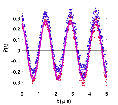
This can be done if the constant {$\alpha$} is obtained independently on the same sample (any small readjustment of the sample position or of the beam transpost may actually vary appreciably this parameter). This is achieved by running a short experiment in a low transverse field {$H$} in a non magnetic phase (if available), in order to have the whole polarization precess in the plane where the two groups lie. The correct value of {$\alpha$} will produce a purely precessing polarization, {$P(t)=A\cos\gamma_\mu H t$}, oscillating around a zero baseline, as shown on the right.
|
{$\alpha$} calibration: the red dots are simulated data, low statistics (as obtained typically counting for few minutes), processed according to Eq. 4, with the correct value of {$\alpha$}; the magenta solid line is the best fit; the blue dots are the same data processed with a value of {$\alpha$} offset by 0.14.
|
Top
|
Signal-to-noise ratio
We are dealing with digital counts from particle detectors within a given time bin, ideally
{$ (1) \qquad\qquad N(t_i)=N_0 e^{-t_i/\tau} \left [1+AP(t_i;\theta)\right] $}
where {$\theta$} is the angle between the direction of the detector axis wand the initial muon spin direction and {$t_i$} is the digitized time interval between implantation time {$t=0$} and positron detection time. Therefore Poisson statistics applies and, if the probability of {$N(t_i)$} being zero is sufficiently low, we expect a standard deviation equal to {$\sqrt{N(t_i)}$}, which we take as the noise level (with 64% confidence).
|
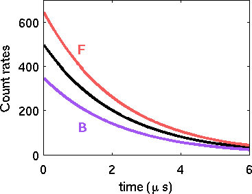
The picture shows three ideal count rates: from a Forward detector (violet), Backward detector (red), unpolarized detector (e.g. at right angles with the (fixed) spin direction.
Top
|
|
Uncorrelated background subtraction
Besides the detected positrons from muon decays, Eq. 1, an experimental setup is bound to pick up counts from uncorrelated events, which, according to Poisson statistics, will give an additional count rate
{$ (2) \qquad\qquad N_u(t_i)= N_{0u} e^{-t/T_u}\quad,$}
but, if the rate {$ T_u^{-1}$} of such events is low enough, it will appear as a constant uncorrelated background, {$N_{0,u}$}. Since we count the sum of Eq. 1 and 2 what really matters is the ratio {$B=\frac {N_{0u}} {N_0}$} for each detector.
Typical figures are:
- {$B=0.01$} on GPS, normal mode, mostly due to beam particles not correctly identified in the spectrometer;
- {$B=10^{-5}$}, virtually unmeasurable, on MUSR, since the beam is pulsed and no particles are transported during the measuring time
- a figure comparable with the latter on GPS with MORE (see the GPS manual for details).
A rather standard procedure is to get the best estimate of this rate and to subtract it from the experimental count rate for the subsequent analysis (however track must be kept of {$N_{0u}$} for the correct estimate of the statistical noise).
|
From the GPS manual, p.62, v. march_2005. Notice that this plot is on a semilog scale. The early times illustrate also a typical measurement on Ag, a standard µSR sample that allows the calibration of the maximum experimental asymmetry, A. Often the sample itself allows this calibration.
|
< Setup | Index | Data analysis: an introduction >
|