• View
• Edit
• History
• Print

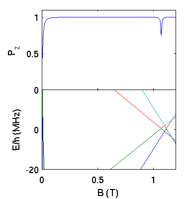
LevelCrossingSimulation

< Avoided Level Crossing (ALC) | Index | How to experimentally detect ALC >

ΔM=0 resonances: hyperfine couplings with other nuclei

The ingredients for this simulation are already contained in the code for the quenching curve. If we calculate the longitudinal time dependent polarization {$P_z(t)$} according to Eq. 1 the constant term originating from {$\langle m|\sigma_{z,\mu}| m \rangle$} will show ALC drops whenever two eigenstates mix around a crossing condition. A typical example is from the e-µ-p system that we have simulated as a prototype radical. This is already provided by the code we have supplied to simulate the longitudinal field polarization.

The picture shows the ALC polarization (top) and a blow-up of the energy levels (bottom) for the e-µ-p system, with {$\nu_0=300 $} MHz, {$\nu_{0p}=100$} MHz. The levels producing the ALC are those originated by the two nuclear replicae of {$\nu_1,\nu_2$} in the equivalent e-µ system. Actually a factor {$\frac {\gamma_e} 2 B$} has been subtracted from these levels, whose slope would otherwise completely hide their small difference around the crossing (notice the MHz scale on the y-axis).

This ALC resonance occurs with a change {$\Delta M=0$} of the z component of the total angular momentum, which is conserved at high fields, This corresponds to a {$\Delta m=\pm 1$} transition for the µ and a {$\Delta m=\mp 1$} transition for the proton. Therefore we must expect one such resonance per

The two terms in the radical Hamiltonian, {${\cal H} + {\cal H}_n$}, are given respecively by , Eq. 1, muonium and Eq. 1, radical. In zeroth order high field approximation, i.e. keeping only the terms in the z spin components, it is straightforward to calculate the value of the crossing field.

{$ \qquad \qquad B_{cr}=\frac {\nu_0-\nu_{0p}} {2(\gamma_\mu-\gamma_p)} $}

which is typically in n the range of the Tesla, and from a few tens to a hundred G off the more accurate matlab result.

ΔM=1 resonances: the case of the anisotropic radical

We have seen that the Hamiltonian for anisotropic radical may be treated in high field approximation as that of muonium, with a reduced hyperfine and an additional hyperfine contribution, the so-called pseudodipolar traceless tensor which represents the dipolar interaction with the electron, averaged over its wave function. In particular this additional contribution will contain the following a term {$ \delta\nu_{z} I_zS_z$} and terms of the kind {$ \delta\nu_{zx} I_zS_x$}.

To illustrate this example we show the numerically simulated muon constant longitudinal polarization (left) and the energy levels (right) vs. applied field, for the following model Hamiltonian {$ \qquad\qquad \frac {\cal H} h = - \gamma_\mu B I_z + \gamma_e B S_z + \nu_0 \mathbf{I}\cdot\mathbf{S} + \delta\nu_z I_zS_z + \delta\nu_{zx} I_zS_x $} which we have simulated with {$\nu_0= 500$} MHz, {$\delta\nu_z=-100$} MHz and {$\delta\nu_{zx}=1$} MHz. It is visible also by the color codes that the two upper triplet states do not cross at {$B_{cr}=4.1\,\mbox{mT}\approx\frac {\delta\nu_z}{\gamma_e-\gamma_\mu}$}, but repel each other, giving rise to a mixing that corresponds to a loss of muon polarization.

< Avoided Level Crossing (ALC) | Index | How to experimentally detect ALC >