< Paramagnetic species | Index | Muonium detailed calculation >
{$$\nu_0=\frac {2\mu_0} {3\pi}\frac {\gamma_\mu\gamma_e\hbar} {\pi a_B^3} $$}
{$$ \quad = 4.46 \cdot 10^9\,\mbox{Hz}$$}
with
{$$\frac {\gamma_\mu} {2\pi} = 1.355\cdot 10^{8}\,\mbox{s/T}$$}
{$$\frac {\gamma_e}{2\pi}= -2.803\cdot 10^{10}\,\mbox{s/T}$$}
{$$a_B=0.532\cdot 10^{10}\,\mbox{m}$$}
Note, aB is slightly larger for Mu.
Muonium is the muon equivalent of the hydrogen atom. When free muonium is formed in its 1s ground state, the muon spin interacts with that of the bound electron, governed by the hyperfine Hamiltonian {$\cal H$}:
{$$ (1) \qquad\qquad \frac {\cal H} h = -\left[ \nu_\mu I_z - \nu_e S_z - \nu_0 \mathbf{I}\cdot\mathbf{S} \right] $$}
where {$2\pi\nu_\mu=\gamma_\mu B$}, {$2\pi\nu_e=|\gamma_e| B$} are the muon and electron Larmor frequencies, due to the Zeeman interaction with the magnetic field, and {$2\pi\nu_0=\frac {2\mu_0} 3 \gamma_\mu|\gamma_e|\hbar|\psi(0)|^2$} is the hyperfine frequency, proportional to the square modulus of the electron wave function {$\psi$} at the muon positition. Eq. (1) explicitly shows the relative signs of the three terms, due to the negative charge of the electron, hence to its negative gyromagnetic ratio (classically, e/2m).
|
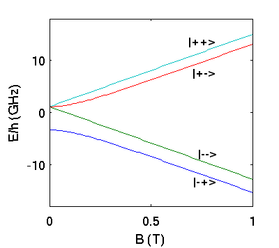
The energy levels of this spin Hamiltonian, a 4x4 matrix, are very easy to recognize for {$B=0,$} since the hyperfine term is invariant under rotations and the addition of the two angular momenta {$I,S=\frac 1 2$} yields two eigenstates: the triply degenerate {$J=1$} state (triplet) and the non-degenerate {$J=0$} state (singlet).
The diagonalization in the general case is not too difficult to perform. We show below a matlab program that does it. The field dependence of the frequencies is plotted on the right (recalling that {$\gamma_e/2\pi=27.992$} GHz/T and {$\nu_0=4.463 302 776(51)$} GHz [1]). For {$B\gt\frac {2\pi\nu_0} {\gamma_e}$} the electron and muon states are decoupled and become as labelled in the plot (electron first).
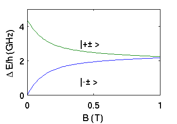
It is easy to see that in this high field regime the two allowed muon transitions are between states of equal electron spin polarization (selection rule {$\Delta m=1$} for the muon only, since µSR detects only muon precessions). Their field dependence is shown on the right, below with a label indicating for each the the two states involved in the transition.
The details of the calculation of frequencies and amplitudes is given in the next page.
|
|
|
Matlab program for muonium energy levels
 sx=[0 1;1 0]; % Pauli matrices definition
 sy=[0 -i;i 0];
 sz=[1 0; 0 -1];
 z=[0 0;0 0];
 o=[1 0; 0 1];
 Iz=[sz z; z sz]/2;% spin matrices  in tensor space e x mu
 Ix=[sx z;z sx]/2;
 Iy=[sy z; z sy]/2;
 Sz=[o z;z -o]/2;
 Sx=[z o;o z]/2;
 Sy=i*[z -o;o z]/2;
 B=0:0.010:1; % up to 1 T
 gamu=135.5; % MHz/T, this is gamma/2 pi
 gae=-27992; % MHz/T
 wm=gamu*B;
 we=gae*B;
 w0=-4400; % MHz hyperfine frequency (nu, not omega)
 w=zeros(length(B),4);
 for k=1:length(B)
    H=-(wm(k)*Iz+we(k)*Sz+w0*(Ix*Sx+Iy*Sy+Iz*Sz)); % Hamiltonian
    w(k,:)=eig(H)';
 end
 plot(B,w/1000); % plots Breit-Rabi levels;
|
|
[1] W. Liu et al., Phys. Rev. Lett. 82, 711 1999.
< Paramagnetic species | Index | Muonium detailed calculation >