< How to detect muonium | Index | Anisotropic muonium state >
The free radical differs from free muonium in that the unpaired electron wave function is delocalized over many more nuclei, several of which possess a spin. Furthermore the electron wave function is not spherically symmetric any more around each of these nuclei, including the muon, as it was in the case of the 1s ground state of muonium. This brings in two modifications to the Hamiltonian of Eq. 1, previous page: the hyperfine coupling becomes a tensor (its trace is the isotropic hyperfine coupling, whereas the traceless tensor is the pseudodipolar contribution), and there are additional terms:
{$$ \begin{equation} \frac {{\cal H}_n} h= - \nu_n I_{nz} - \mathbf{ I}_n\cdot\nu_{0n}\cdot\mathbf{S} \end{equation}$$}
|
for each nucleus in the molecule, with spin {$I_n$}. The Hamiltonian of Eq. 1 quickly grows in dimensions, equal to
{$$2^2\cdot N=4\prod_{n=1}^m(2I_n+1)$$}
with the number {$m$} of nuclei involved. However it is still rather simple to obtain the muon transitions in the high field condition, the so-called Paschen-Bach regime where {$B\gt\mbox{max}\{\omega_0,\omega_{0n}\}/\gamma_e$}. In this regime all the spins are decoupled and the eigenvalues of {$I_z,S_z,I_{nz}$} are good quantum numbers. Therefore the measurement of {$I_x$} can induce only muon spin transitions, whereas all other quantum numbers must remain constant. In practice one has {$N$} replicae of the corresponding muonium-like energy levels, determined only by the muon and electron spin.
The plot on the right is obtained with one additional proton and hyperfine frequencies {$\nu_0=500 $} MHz and {$\nu_{op}=150$} MHz, as appropriate for the cyclohexadienyl radical obtained by Mu addition to benzene (although that radical actually has six hydrogens.
|
|
|
|
Allowing for a hyperfine traceless anisotropy tensor {$\delta\tilde\nu_0$} one has an effective Hamiltonian:
{$$\begin{equation} \frac {\cal H} h = - \left[ \nu_\mu I_z - \nu_e S_z + \mathbf{I}\cdot(\nu_0+\delta\tilde\nu_0)\cdot\mathbf{S} \right] \end{equation}$$}
valid only at high fields. The tensor {$\delta\tilde\nu_0$} can be written as:
{$$ \delta\tilde \nu_0= \delta\nu_0 \left(\begin{array}-\frac 1 2 & 0 & 0 \\ 0 & -\frac 1 2 & 0 \\ 0 & 0 & 1\end{array}\right)$$}
in the reference frame of its principal axes, {$\xi,\eta$}.
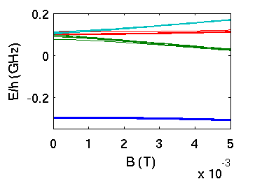
The plot on the left shows the spread in the levels obtained at relatively low field (where also nuclear hyperfines would complicate further the picture) by rotating around a randomly chose axis with the following hyperfine paramenters: {$\nu_0=400 \mbox{MHz}$} and {$\delta\nu_0=30 \mbox{MHz}$}.
|
|
The observation of narrow muon transitions requires either a single crystal, to select the tensor orientation, or a liquid, to average out the effects of the anisotropy by fast reorientation. The last case reduces Eq. 2 to the isotropic muonium Eq. 1, previous page, just with a reduced value of isotropic hyperfine frequency {$\omega_0$}.
A radical in a liquid at high fields then shows two precession frequencies:
{$$ \begin{eqnarray} \nu_{12} &\approx &\nu_0/2 + \frac{\gamma_\mu} 2 B\\ \nu_{34} &\approx &-\nu_0/2 + \frac{\gamma_\mu} 2 B\end{eqnarray} $$}
so that their difference is equal to {$\nu_0$} and their sum approximately equal to {$\gamma_\mu B$}.
For a more complete account of radical chemistry aspects see E. Roduner, Springer-Verlag, Berlin (1988).
< How to detect muonium | Index | Anisotropic muonium state >