< a collection of python hints | Index | Install Musrfit >
The Minuit python port is iminuit
For the moment only PyMinuit works, not PyMinuit2, follow http://code.google.com/p/pyminuit/wiki/HowToInstall and see here for some more details. Below, I assume one has python, ipython, Minuit1.7.9 and PyMinuit installed. The bottom lines assume also the availability of matplotlib.
Usage of PyMinuit is mostrly explained in Getting started and Function Reference
The logic to follow is explained in this most important Python FAQ. Let's assume we want to perform an interactive fit of some experimental data to a Gaussian peak, in the style of the fminuit demo, from Giuseppe Allodi. So we are working from a Unix terminal
- start ipython
- import minuit
- in order to pass data to pyminuit we need a
mu_cfg.py script like
from __future__ import division # this is to avoid surprises
# from integer divisons
data=np.c_[np.arange(0.,5.,0.01),
5.*np.exp(-(((np.arange(0.,5.,0.01)-2.8)/0.7)**2/2.)
+0.2*np.random.standard_normal(np.size(np.arange(0.,5.,0.01))),
0.2*np.ones(np.size(np.arange(0.,5.,0.01)))]
# this is a fake set of data, in the form of an nx3 matrix
# first row: independent variable (say frequency)
# second row: data
# third row: uniform expected standard deviations
- write a fitting routine with separate function and chi2 calculation
and save it as, e.g., gauss.py
from __future__ import division
import numpy as np
import mu_cfg as mu # very important!
def f(p1,p2,p3):
'''Gaussian function of
of amplitude p(1), center p(2) and sigma p(3)
'''
f=p1*np.exp(-(((mu.data[:,0].copy()-p2)/p3)**2)/2)
return f
def chi2(p1,p2,p3):
"""Sum of the square deviations of mu.data, whose
second row contains data, from f, when the third row is empty;
normalized sum of square deviations,
when the third row of mu.data contains standard deviations.
"""
if np.size(mu.data,0)==2:
chi2=np.sum((mu.data[:,1].copy()-f(p1,p2,p3))**2)
elif np.size(mu.data,0)>2:
chi2=np.sum(((mu.data[:,1].copy()-f(p1,p2,p3))/mu.data[:,2].copy())**2)
return chi2
- Now fit the data from the interactive terminal, as follows
import mu_cfg as mu
m=minuit.Minuit(gauss.chi2,p1=2.,p2=2.1,p3=1.2),
choosing starting values near the right values
m.migrad()
m.hesse()
m.values
prints the fitted parameter values
m.errors
prints the standard deviations
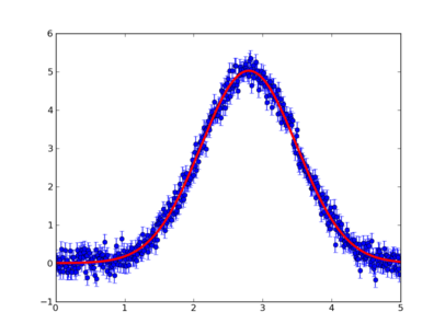
errorbar(mu.data[:,0].copy(),mu.data[:,1].copy(),yerr=mu.data[:,2].copy(),fmt='o')
plot(mu.data[:,0].copy(),gauss.f(*m.args),'r-',linewidth=3)
produces the following
< a collection of python hints | Index | Install Musrfit >