< Precession in the muonium state | Index | How to detect muonium >
The muon polarization in a given direction {$\xi$} is obtained as the average value of the muon spin in that direction, normalized to the muon spin itself. This amounts to calculating the average of the muon Pauli matrix {$\sigma_{\mu\xi}$}:
{$$ (1)\qquad\qquad P_{\xi\eta}(t) = Tr \rho_0(t)(\sigma_{\mu\xi}\otimes1_e) $$}
If the electron and muon initially are respectively unpolarizad and polarized along {$\eta$} the density matrix is given by:
{$$ (2a)\qquad\qquad \rho_0 = \frac 1 4 (1_\mu+\sigma_{\mu\eta}) \otimes \,1_e $$}
The factor 1/4 on the right hand side gives the correct normalization, remembering that {$Tr \rho_0$} must be unity.
In the averages like Eq. (1) one may use directly
{$$ (2b)\qquad\qquad \rho^\prime_0 = \frac 1 4 \sigma_{\mu\eta} \otimes \,1_e$$}
since {$Tr \sigma_{\mu\xi} \otimes 1_e =0$}. Let us consider the matrix expressed in the reference set where {$\sigma_{\mu\eta}$} is diagonal
{$$ \sigma_{\mu\eta}=\begin{bmatrix} 1 & 0\\ 0 &-1\end{bmatrix}$$}
|
Define the first state as that of the electron :
{$$ |+\, +\rangle = \begin{bmatrix} 1\\0\\0\\0\end{bmatrix}; \qquad |+\, -\rangle = \begin{bmatrix} 0\\1\\0\\0\end{bmatrix}; \qquad |-\, +\rangle = \begin{bmatrix} 0\\0\\1\\0\end{bmatrix}; \qquad |-\, -\rangle = \begin{bmatrix} 0\\0\\0\\1\end{bmatrix}$$}
|
so that the explicit form of the full density matrix, Eq. (2), is:
{$$ \rho_0= \frac 1 2 \begin{bmatrix} 1& 0& 0& 0\\ 0& 0 & 0& 0\\ 0& 0& 1& 0\\ 0& 0& 0& 0 \end{bmatrix} $$}
This density tells us that only spin-up muon states along {$\eta$} are initially occupied. For the calculations however we shall use Eq. (2b)
|
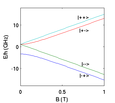
We have already obtained the muonium hamiltonian eigenvalues in a field, by matlab diagonalization. Let's rewrite the hamiltonian matrix:
{$$ (3a)\qquad\qquad \frac {\cal H} h = \quad \begin{bmatrix}\frac {\nu_0} 4 \,+\, \frac{\nu_-} 2& 0& 0& 0\\ 0&-\frac {\nu_0} 4\, + \,\frac {\nu_+} 2 & -\frac {\nu_0}2 & 0\\ 0& -\frac {\nu_0}2& -\frac {\nu_0}4\,-\,\frac {\nu_+}2& 0\\ 0& 0& 0& \frac {\nu_0}4\,-\,\frac{\nu_-} 2 \end{bmatrix} $$}
and the analytical expression for the eigenvalues is easy to find, since there is only one 2x2 block:
{$$ (3b)\qquad\qquad \begin{eqnarray*}\nu_1 &=& \frac {\nu_0} 4 + \frac{\nu_-} 2 \\ \,&\\ \nu_2 &=&-\frac {\nu_0} 4 (1-2\sqrt{1+x^2})\\ \, &\\\nu_3 &=& -\frac {\nu_0} 4 (1+2\sqrt{1+x^2})\\ \,&\\ \nu_4 &=& \frac {\nu_0} 4 -\frac{\nu_-} 2 \end{eqnarray*} $$}
where {$ \nu_-=\frac 1 2(|\gamma_e| -\gamma_\mu)B,\quad \nu_+=(|\gamma_e| +\gamma_\mu)B$} and {$ x= \nu_+/\nu_0$}.
If we define {$B_0=\frac{\nu_0} {|\gamma_e|+\gamma_\mu}$} the fraction x is the ratio B/B0 . Considering that |γe|/2π = 28.025 GHz/T, we can introduce the constant Γ=(|γe|-γμ)/(|γe|+γμ)=0.9904, very close to 1 and rewrite directly the pulsations ω
{$$ (3c)\qquad\qquad \begin{eqnarray*}\omega_1 &=& \frac{\omega_0} 4 \left( 1+ 2\Gamma x\right) \\ \,&\\ \omega_2 &=&-\frac {\omega_0} 4 \left(1-2\sqrt{1+x^2}\right)\\ \, &\\ \omega_3 &=& -\frac {\omega_0} 4 \left(1+2\sqrt{1+x^2}\right)\\ \,&\\ \omega_4 &=& \frac{\omega_0} 4\left( 1 - 2 \Gamma x\right) \end{eqnarray*} $$}
The eigenvectors can be readily calculated as
{$$ (4)\qquad\qquad \begin{eqnarray*}| 1\rangle &=& | +\, +\rangle; \\ | 2\rangle &=& s| +\, -\rangle + c| -\, +\rangle; \\ | 3\rangle &=& c| +\, -\rangle -s| -\, +\rangle; \\ | 4\rangle &=& | -\, -\rangle \end{eqnarray*}$$}
with
{$$ (5)\qquad\qquad s,c = \frac 1 {\sqrt 2}\sqrt{1\pm\frac x {\sqrt{1+x^2}}} $$}
|
The triplet states are 1,2,4 and the singlet is 3. This sequence coincides with the ordering from the top at intermediate fields (below {$B_x=\omega_0/2\gamma_\mu=16.47$} T, the field where 1 and 2 are degenerate). Above {$B_x$} the order from the top becomes 2,1,4,3.
|
Now, in order to compute the time dependent Heisenberg operator in Eq. 1, e.g. {$\rho(t)$}, we need the time evolution operator:
{$$U(t)=e^{-i2\pi {\cal H} t/h} $$}
which, in the base of the eigenvectors of {$\cal H$}, has matrix elements {$\langle j |U(t)| k\rangle = e^{-i2\pi \nu_k t}\delta_{jk} $}. Then with implicit summation of all double indices Eq. 1 may be rewritten as:
{$$ (6)\qquad\qquad \begin{eqnarray*} P_{\xi\eta}(t) &=& \frac 1 4 \ e^{-i2\pi (\nu_n-\nu_k) t}\delta_{jk}\delta_{mn} \langle k |\sigma_{\mu\eta}\otimes1_e| m\rangle \langle n |\sigma_{\mu\xi}\otimes1_e| j\rangle \\&=& \frac 1 4 \ e^{-i2\pi (\nu_n-\nu_k) t} \langle k |\sigma_{\mu\eta}\otimes1_e| n\rangle \langle n |\sigma_{\mu\xi}\otimes1_e| k\rangle \end{eqnarray*}$$}
|
We have now to specialize to specific cases. Often one observes the muon precession along the polarization direction, either in longitudinal or in transverse fields, i.e. {$\xi=\eta=z$} or {$\xi=\eta=x$}.
The first case is very simple to calculate, since
{$$ \begin{eqnarray*}|\langle 1 |\sigma_{\mu z}\otimes1_e| 1\rangle|^2 &=& |\langle 4 |\sigma_{\mu z}\otimes1_e| 4\rangle|^2& =&1; \\ |\langle 2 |\sigma_{\mu z}\otimes1_e| 2\rangle|^2 &=&|\langle 3 |\sigma_{\mu z}\otimes1_e| 3\rangle|^2&=&(s^2-c^2)^2; \\ &&|\langle 2 |\sigma_{\mu z}\otimes1_e| 3\rangle|^2 &=& 4c^2s^2\end{eqnarray*}$$}
are the only non vanishing matrix elements. This gives
{$$ (7) \qquad\qquad \begin{eqnarray*} P_{zz}(t)&=& s^4 + c^4 + c^2s^2 (e^{-i2\pi (\nu_2-\nu_3) t}+ e^{-i2\pi (\nu_3-\nu_2) t})\\ &=& \frac 1 {2(1+x^2)} \left(1+2x^2 + cos2\pi (\nu_2-\nu_3) t\right)\end{eqnarray*}$$}
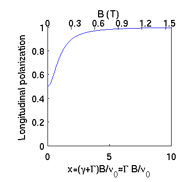
Notice that the frequency {$\nu_2-\nu_3=\nu_0$} has amplitude {$\frac 1 2$} at {$B=0; x=0$}, but it is very difficult to observe directly for pure muonium (4.4 GHz requires at least 100ps digitizing resolution), hence simple spectrometers generally detect only the constant term
{$$ P_{zz}(t)= \frac{1+2x^2}{2(1+x^2)} $$}
shown in the right figure
|
Longitudinal field initial polarization, {$P_z(t=0)$}, the so-called muonium quenching curve, i.e. the constant in Eq. 7.
|
|
Similar calculations, omitting 1e for simplicity,
{$$\begin{eqnarray*} |\langle 1 |\sigma_{\mu x}| 1\rangle|^2 &=& |\langle 2 |\sigma_{\mu x}| 2\rangle|^2 = |\langle 3 |\sigma_{\mu x}| 3\rangle|^2 = |\langle 4 |\sigma_{\mu x}| 4\rangle|^2 &=& 0; \\ |\langle 1 |\sigma_{\mu x}| 2\rangle|^2 &=& |\langle ++ |\frac{\sigma_{\mu +}+\sigma_{\mu -}} 2 \left(s|+-\rangle + c|-+\rangle\right)|^2 &=&s^2; \\ |\langle 4 |\sigma_{\mu x}| 3\rangle|^2 &=& |\langle -- |\frac{\sigma_{\mu +}+\sigma_{\mu -}} 2 \left(c|+-\rangle - s|-+\rangle\right)|^2 &=&s^2; \\ |\langle 1 |\sigma_{\mu x}| 3\rangle|^2 &=& |\langle ++ |\frac{\sigma_{\mu +}+\sigma_{\mu -}} 2 \left(c|+-\rangle - s|-+\rangle\right)|^2 &=&c^2; \\ |\langle 4 |\sigma_{\mu x}| 2\rangle|^2 &=& |\langle -- |\frac{\sigma_{\mu +}+\sigma_{\mu -}} 2 \left(s|+-\rangle + c|-+\rangle\right)|^2 &=&c^2; \\ |\langle 2 |\sigma_{\mu z}| 3\rangle|^2 &=& 0\end{eqnarray*}$$}
lead to
{$$ \begin{align*} P_{xx}(t)& =\frac 1 4 \left[ s^2 \left(e^{-i2\pi (\nu_1-\nu_2) t} +e^{-i2\pi (\nu_2-\nu_1) t} + e^{-i2\pi (\nu_3-\nu_4) t}+e^{-i2\pi (\nu_4-\nu_3) t}\right) \right. + \\ & \left. c^2\left(e^{-i2\pi (\nu_1-\nu_3) t} +e^{-i2\pi (\nu_3-\nu_1) t} + e^{-i2\pi (\nu_2-\nu_4) t}+e^{-i2\pi (\nu_4-\nu_2) t}\right)\right] \\ & =\frac 1 4 \left[(1+\frac{x}{\sqrt{1+x^2}}) \left(cos2\pi(\nu_1-\nu_2)t + cos2\pi(\nu_3-\nu_4)t\right)\right. +\\ &\left. (1-\frac{x}{\sqrt{1+x^2}}) \left(cos2\pi (\nu_1-\nu_3) t+cos2\pi(\nu_4-\nu_2)t\right)\right]\end{align*}$$}
We define the transitions {$\nu_{jk}=\nu_j-\nu_k$} and, as it is shown in the right figure
- for {$x(B)\rightarrow 0$} the four amplitudes are s,c = 1/4;
- for {$x(B)\rightarrow \infty$} the amplitudes of the 12, 34 transitions survive, {$s\rightarrow 1 $}, and those of the 13, 24 transitions, c, vanish .
|
Transverse field precessing amplitudes of the oscillating terms in Eq. 8
|
The two high field transition frequencies are:
{$$ (9) \qquad\qquad \nu_{12,34} = \frac 1 2 ( \nu_0 \pm \nu_{-} \, \mp \sqrt{\nu_0^2 + \nu_{+}^2}) $$}
that, for B>>B0 , become
{$$ (10) \qquad\qquad \nu_{12,34} = \frac {\nu_0} 2 \mp \nu_\mu \mp \frac 1 4 \frac {\nu_0^2}{\nu_+} $$}
so that their sum is {$\nu_0$} and their difference in first approximation is {$2\gamma_\mu B$}. Keep in mind that when {$\nu_{12}$} becomes negative the sum and the difference of the observed frequencies are interchanged.
< Precession in the muonium state | Index | How to detect muonium >