Unpolarized muonium

We add here another exercise: isotropic muonium (i.e. Mu formed with an unpolarized electron, and stopping in a magnetic enviroment) in an internal field B_d , along a local direction z. The Hamiltonian, eigenstates and eigenvalues are those of muonium, Eqs. (3), (4) and (5). Think of B_d as a classical external field, the mean dipolar field produced by distant dipoles over the region occupied by Mu. Note that the internal field of the 1s electron on the muon, 2πν₀/γ_μ, is roughly 150 mT and as long as the internal field of the magnetic environment is larger than 150 mT the weights in those equations are s~1 and c~0. We must now compute the longitudinal polarization

{$$P_{\eta\eta}(\theta, t)=Tr\rho_0(t)\sigma_{\mu,\eta}$$}

with a density matrix appropriate for the muon spin is initially along η: {$\rho^{'}_0 = \sigma_{\mu\eta}\otimes 1_e/4$}. We now wish to compute Eq. (6) of muonium with {${\hat\eta}\cdot{\hat z}=cos\theta$}. Mu is isotropic but B_d breaks rotational symmetry in a single crystal, single domain sample. Polycrystalline average over θ recovers rotational symmetry.

We can rewrite {$\sigma_{\mu\eta}=\cos\theta\sigma_{\mu z}+\sin\theta\sigma_{\mu x}$} and, dropping the 1_e operator, calculate le polarization for observation along the initial muon direction η (longitudinal case)

{$$ \begin{align*} P_{\eta\eta}(t) &= \frac 1 4 \ e^{-i2\pi (\nu_n-\nu_k) t}\delta_{jk}\delta_{mn} \langle k |\sigma_{\mu\eta}| m\rangle \langle n |\sigma_{\mu\eta}| j\rangle \\&= \frac 1 4 \ e^{-i2\pi (\nu_n-\nu_k) t} |\langle k |\sigma_{\mu\eta}| n\rangle|^2 \end{align*}$$}

With the singlet and triplet eigenstate coefficients s(x), c(x) as defined in muonium, Eq. (5), and the matrix elements already calculated there

we get

{$$ \begin{align*} P_{\eta\eta}(\theta,t) &= \frac 1 2 \left( \cos^2\theta\, \left[ 1+(s^2-c^2)^2 + 4s^2c^2 \cos\omega_{23} t\right] \right. \\ & +\left. \sin^2\theta\,\left[s^2 \left(cos\omega_{21}t + \cos\omega_{34}t\right)\right.\right.\\ & + \left.\left.\, c^2 \left( \cos\omega_{31}t+\cos\omega_{24}t \right)\right] \right) \\ & \approx \cos^2\theta + \frac 1 2 \,\sin^2\theta \left(\cos\omega_{21}t+\cos\omega_{34}t\right) \end{align*}$$}

The exact function is

{$$\begin{align*}P_{\eta\eta}(\theta,x,t) &= \cos^2\theta \frac 1 2 \left[ 1+\frac {x^2} {1+x^2} + \frac 4 {1+x^2} \cos\omega_{23} t\right] \\&+ \frac 1 4 \,\sin^2\theta\,\left[ \left(1+\frac x {\sqrt{1+x^2}}\right)(cos\omega_{21}t + \cos\omega_{34}t)\right.\\ & +\, \left.\left(1-\frac x {\sqrt{1+x^2}}\right) (\cos\omega_{31}t+\cos\omega_{24}t)\right]\end{align*}$$}

with the following transitions

{$$\omega_{23}=\frac {\omega_0} 2 \\ \omega_{21}=\frac {\omega_0} 2\left(1 - \Gamma x + \sqrt{1+x^2} \right)\\ \omega_{31}=\frac {\omega_0} 2\left(1 - \Gamma x - \sqrt{1+x^2} \right)\\ \omega_{24}=\frac {\omega_0} 2\left(1 + \Gamma x + \sqrt{1+x^2} \right) \\ \omega_{34}=\frac {\omega_0} 2\left(1 + \Gamma x - \sqrt{1+x^2} \right)$$}

If we take the powder average over θ the unpolarized muonium pattern in sufficiently high local fields is given by 1/3 non precessing term plus two further 1/3 terms precessing at {$\frac {\nu_0} 2 \,(1\,\,\mp\,\,\sqrt{1+x^2} \,\,\pm\,\, \Gamma x)$}. The extrema in the figures on the right (minimum of B₁₂ , maximum of B₃₄ ) happen very close to T_c , for

{$x_m = \frac {B_d}{B_0}(1-t)^\beta=\frac \Gamma {\sqrt{1-\Gamma^2}}=\frac{\gamma_e-\gamma_\mu}{2\sqrt{\gamma_e\gamma_\mu}}=7.156$}

In the two plots this happens respectively for T/T_c -1 = 0.01, 0.0001 for B₀ = 15, 3.4 mT

Blue: internal field. Red, green, local muon fields at Mu with ν₀ = 440MHz

Same with ν₀ = 100 MHz

local index

Polarized muonium

If muonium however is formed with an electron thermalized at the Fermi level of the magnetic material, it may be polarized. In a half metal at low temperature it would be 100% polarized. We must compute its polarization as

{$P_{\eta\eta}(\theta, t)=Tr\rho_{0\uparrow\downarrow}(t)\sigma_{\mu,\eta}$}

with a density matrix appropriate for the muon spin is initially along η and the electron spin along ±z:

{$\rho_{0\uparrow\downarrow}=\frac 1 4 \left(1_e\pm\sigma_{ez}\right)\otimes\left(1_\mu +\sigma_{\mu\eta}\right) = \frac 1 4 \left( 1_e\otimes 1_\mu + 1_e\otimes\sigma_{\mu\eta} \pm \sigma_{ez}\otimes 1_\mu \pm \sigma_{ez}\otimes\sigma_{\mu\eta} \right)$}.

Dropping the big identity because it does not contribute to the trace and the other identities for simplicity we obtain ρ_±=σ_μη ± σ_ez ± σ_ezσ_μη. We may therefore write

{$P_{\eta\eta}(\theta, t)= \frac 1 4 \sum_{mn=1}^4 e^{i\omega_{mn}t}\left[|\langle m|\sigma_{\mu \eta}|n\rangle|^2 \pm \langle m|\sigma_{ez}|n\rangle\langle n|\sigma_{\mu \eta}|m\rangle \pm \langle m|\sigma_{ez}\sigma_{\mu \eta}|n\rangle\langle n|\sigma_{\mu \eta}|m\rangle\right]$}

and in the sum of the first term in square parenthesis we recognize the result for unpolarized Mu. We must now work out the sum of the second and of the third term, corresponding respectively to the first and second line below

{$\pm\cos\theta\langle m|\sigma_{ez}|n\rangle\langle n|\sigma_{\mu z}|m\rangle\pm\sin\theta\langle m|\sigma_{ez}|n\rangle\langle n|\sigma_{\mu x}|m\rangle \\ \pm\cos^2\theta\langle m|\sigma_{ez}\sigma_{\mu z}|n\rangle\langle n|\sigma_{\mu z}|m\rangle \pm \sin^2\theta\langle m|\sigma_{ez}\sigma_{\mu x}|n\rangle\langle n|\sigma_{\mu x}|m\rangle \pm \sin\theta\cos\theta\left(\langle m|\sigma_{ez}\sigma_{\mu z}|n\rangle\langle n|\sigma_{\mu x}|m\rangle+\langle m|\sigma_{ez}\sigma_{\mu x}|n\rangle\langle n|\sigma_{\mu z}|m\rangle\right)$}

By direct inspection we recognize that the products with a single matrix element of σ_µx vanish, leaving only the following three new terms

{$ \pm \cos^2\theta\langle m|\sigma_{ez}\sigma_{\mu z}|n\rangle\langle n|\sigma_{\mu z}|m\rangle \pm \sin^2\theta\langle m|\sigma_{ez}\sigma_{\mu x}|n\rangle\langle n|\sigma_{\mu x}|m\rangle \pm \cos\theta\langle m|\sigma_{ez}|n\rangle\langle n|\sigma_{\mu z}|m\rangle $}

The first also vanishes, while the second selects either the 12 and 13 transitions or the 23 and 24 transitions of the unpolarized Mu. Adding finally the third term we obtain the new total function

{$ \begin{eqnarray} P_{\eta\eta\uparrow}(\theta,t) &=& \frac 1 2 \cos^2\theta\,\left[1 +(s^2-c^2)^2 + 4s^2c^2 \cos\omega_{23} t\right] \\ && + \,\sin^2\theta\,\left[s^2 \cos\omega_{21}t + \, c^2 \cos\omega_{31}t \right] \\ &&+ \frac 1 2 \cos\theta\left[ 1 -(s^2-c^2)^2 - 4s^2c^2 \cos\omega_{23} t \right]\end{eqnarray}$}

{$ \begin{eqnarray} P_{\eta\eta\downarrow}(\theta,t) &=& \frac 1 2 \cos^2\theta\,\left[1 +(s^2-c^2)^2 + 4s^2c^2 \cos\omega_{23} t\right] \\ && + \,\sin^2\theta\,\left[s^2 \cos\omega_{34}t + \, c^2 \cos\omega_{24}t \right] \\ &&- \frac 1 2 \cos\theta\left[ 1 -(s^2-c^2)^2 - 4s^2c^2 \cos\omega_{23} t \right]\end{eqnarray}$}

If we take the powder average over θ (<cos² θ> = 1/3, <sin² θ> =2/3, <cosθ> = 0), the majority spin polarized muonium pattern in high local fields (s terms are 1 and c terms vanish) is given by

{$ \begin{eqnarray} P_\uparrow(t) &=& \frac 1 3 \left[ 1+ 2cos\omega_{12}t \right] \end{eqnarray}$}

corresponding to a precession around B_d with muonium electron spin up. If we start from the minority spin, with density matrix {$\rho_{0\downarrow}$} we obtain

{$ \begin{eqnarray} P_\downarrow(t) &=& \frac 1 3 \left[ 1+ 2cos\omega_{34}t \right] \end{eqnarray}$}

corresponding to a precession around B_d with muonium electron spin down.

local index

Electron spin-flip scattering

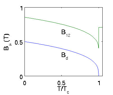
Looking at the polarized Mu results we can deduce what happens upon electron spin-flip scattering. Usually electron scattering times τ_e are much shorter than spin precession periods, i.e in the motional narrowing limit, with electron rate τ_eω_e; << 1. In the strong collision limit (unitary scattering, a spin-flip for every electron collision) the constant longitudinal component is preserved and the oscillating transverse component is averaged to

{$\omega_\mu=\frac {\omega_{12}+\omega_{34}} 2 \approx \frac {\omega_0} 2$}

This average is accompanied by a T₂ relaxation of the transverse component, driven by a modulation of the secular Hamiltonian, of amplitude {$2\gamma_\mu B_d(T)$}. In motional narrowing regime by

{$\frac 1 {T_{2}} = 4\gamma_\mu^2 B_d^2(T) \tau_e$}

The same fluctuation is ineffective in producing a T₁ process, that can only happen in anisotropic Mu.

Fluctuations inverting the local field, {$x\rightarrow -x$}, such as critical fluctuations or muon diffusion, or maybe magnetic polarons, produce the average of ω₁₂ and ω₂₄

{$\omega_\mu=\frac {\omega_{12}+\omega_{24}} 2 \approx \frac {\omega_0} 2 + \frac{\gamma_e+\gamma_\mu} 2 B_d(T)$}

This frequency is unobservably large, roughly 100 times that of a bare muon in the same magnetic material. The relaxation in this case is also much faster (in the order of (γ_e/γ_μ)² = 4.3 10⁴).

{$\frac 1 {T_{2}} = (\gamma_e-\gamma_\mu)^2 B_d^2(T) \tau_e$}

Both cases assume that the Mu electron, if this makes any sense, is not thermalized with the lattice, i.e. it does not belong to a metal electron band. When the latter thing happens B_d and B₀ fluctuate at the same time. One such collision could reverse both the hyperfine coupling (�.e. the Mu electron) and the local field of the other electrons. Let's e.g. take the 12 transition at time t=0. The collision would simultaneously turn eigenstate 1 to 3 and 3 to 2, leading to a change in phase by π. In an external field B fast fluctuations like these average to a precession at ω_μ = γ_μ B .

local index

Spin operators on the eigenstates of Mu

The action of the spin operators on the Mu eigenstates in the matrix elements of the trace is the following, distinguished in a longitudinal part, along z, unpolarized

{$\sigma_{\mu z}|1\rangle = \sigma_{\mu z}|++\rangle=|++\rangle=|1\rangle \\ \sigma_{\mu z}|2\rangle = \sigma_{\mu z}(s|+-\rangle +c|-+\rangle)=-s|+-\rangle + c|-+\rangle = (c^2-s^2)|2\rangle-2cs|3\rangle \\ \sigma_{\mu z}|3\rangle = \sigma_{\mu z}(c|+-\rangle -s|-+\rangle)=-c|+-\rangle - s|-+\rangle = (s^2-c^2)|3\rangle-2cs|2\rangle \\ \sigma_{\mu z}|4\rangle = \sigma_{\mu z}|--\rangle=-|--\rangle=-|4\rangle$}

and polarized

{$\sigma_{e z}\sigma_{\mu z}|k\rangle = |k\rangle, \quad k=1, 4 \\ \sigma_{e z}\sigma_{\mu z}|2\rangle = \sigma_{e z}\sigma_{\mu z}\left(s|+-\rangle + c|-+\rangle\right) = -s|+-\rangle - c|-+\rangle = -|2\rangle \\ \sigma_{e z}\sigma_{\mu z}|3\rangle = \sigma_{e z}\sigma_{\mu z}\left(c|+-\rangle - s|-+\rangle\right) = -c|+-\rangle + s|-+\rangle = -|3\rangle$}

plus a transverse part, unpolarized

{$\sigma_{\mu x}|1\rangle = \sigma_{\mu x}|++\rangle = |+-> \\ \sigma_{\mu x}|2\rangle = \sigma_{\mu x}(s|+-\rangle + c|-+\rangle) = s|++\rangle + c|--\rangle = s|1\rangle + c|4\rangle\\ \sigma_{\mu x}|3\rangle = \sigma_{\mu x}(c|+-\rangle - s|-+\rangle) = c|++\rangle - s|--\rangle = c|1\rangle - s|4\rangle \\ \sigma_{\mu x}|4\rangle = \sigma_{\mu x}|--\rangle = -|-+\rangle $}

and polarized

{$\sigma_{e z}\sigma_{\mu x}|1\rangle = \sigma_{e z}\sigma_{\mu x}|++\rangle = |+-> \\ \sigma_{e z}\sigma_{\mu x}|2\rangle = \sigma_{e z}\sigma_{\mu x}(s|+-\rangle + c|-+\rangle) = s|++\rangle - c|--\rangle = s|1\rangle - c|4\rangle\\ \sigma_{e z}\sigma_{\mu x}|3\rangle = \sigma_{e z}\sigma_{\mu x}(c|+-\rangle - s|-+\rangle) = c|++\rangle + s|--\rangle = c|1\rangle + s|4\rangle \\ \sigma_{e z}\sigma_{\mu x}|4\rangle = \sigma_{e z}\sigma_{\mu x}|--\rangle = |-+\rangle $}

Finally the sole action of σ_ez

{$\sigma_{ez}|1\rangle = |1\rangle \\ \sigma_{ez}|2\rangle = \sigma_{ez}(s|+-\rangle + c|-+\rangle) = s|+-\rangle - c|-+\rangle = (s^2-c^2)|2\rangle + 2sc|3\rangle\\ \sigma_{ez}|3\rangle = \sigma_{ez}(c|+-\rangle - s|-+\rangle) = c|+-\rangle + s|-+\rangle = 2sc|2\rangle +(c^2-s^2)|3\rangle \\ \sigma_{ez}|4\rangle = -|4\rangle $}

local index

< Anisotropic muonium state | Index | How to simulate the radical >

MuoniumPowdersCalculation

Local index

Unpolarized muonium