< mulab main tools | Index | The internal structure of mulab: Globals >
Binning
The main panel allows selection of a Bin. This integer value indicates how many original data points
are rebinned together. For Bin n, n successive asymmetry points are averaged, and taken to correspond
to the mean time of this bin interval. This enhances the signal/noise ratio if the muon asymmetry is composed
of low frequency components. The procedure affects only the display. The fit is always performed over unbinned data.
Top
FFT of residues
By pressing the FFT button in the main panel you can obtain the Fourier Transform of the fit resiudes
The fit is subtracted from the data according to the displayed parameters, so if you want to subtract
the best fit, you must first press the Update button. Partial subtraction may be performed: only the
components with the FFT tick mark set are actually subtracted. The FFT is displayed in a triple plot,
with Power (top), Real part (middle) and Imaginary part (bottom). The colour-shaded area should indicate
signals above noise level (check if behaviour is consistent!).
The main panel allows selection of plot frequency range and apodization window. Signal at times past a chosen
cutoff are strongly damped, The inverse time cutoff is selected as LB (Line Broadening): 1 µs-1 to
match a signal that decays within 1 µs.
From version 1.05 FFT amplitudes can be rephased from the FFT plot window, adding either a constant phase to all
frequencies or a frequency-linear contribution.
If you want to access the fft data the easiest is to type in the command window:
global MU_DATA
then you can see the data as:
MU_DATA.FREQUENCY, frequency vector
MU_DATA.FFTREAL, real part vector
MU_DATA.FFTIMAG, imaginary part vector
MU_DATA.EFFT, error vector
For exporting you can save this as an ascii file with
save -ascii fft.dat [MU_DATA.FREQUENCY;MU_DATA.FFTREAL;MU_DATA.FFTIMAG;MU_DATA.EFFT]
in matlab v. 7, and
save('fft.dat','MU_DATA.FREQUENCY','MU_DATA.FFTREAL','MU_DATA.FFTIMAG','MU_DATA.EFFT','-ascii')
in later versions (2006 onwards)
Top
Linear relations (Ver. 1.05)
In some instances you may wish to force a linear relation among parameters.
Typically you may wish to force that the partial asymmetry of a given precessing component,
'mu', is twice the partial asymmetry of its longitudinal fraction, 'ba'. In this case you
would have a simple 'bamu' model, with 8 parameters, with the following approximate look
in the menu window
 1 - baAmp   0.08   ~      4 - muAmp  0     +p(1)*2
 2 - baDeLo  0.1    ~      5 - muGau  750   ~
 3 - baDeGa  0      !      6 - muPhi  0     ~
                           7 - muDeLo 0     !
                           8 - muDeGa 1.5   ~
The symbol signalling a linear relation is the leading + in the muAmp second input
the syntax in the following string is almost self evident: p(1) indicates baAmp and the index
is that of the Menu. The full string must be an executable matlab assignment, supposing that p is already
assigned as the parameter array. It will be automatically remapped with the internal fminuit parameter indices
and the actual string executed by fminuit may be seen by issuing the following commands, after a succesful fit
 global MU_MODEL_F
 MU_MODEL_F.COMPONENT(2).PARAMETER(1).MENU2MINUIT
where COMPONENT(2) stands for mu and PARAMETER(1) stands for Amp
A more complex string may be used, if it ever made any sense:
+p(1)*2-p(2)/3*4-0.234^2
Top
Shared parameters (Ver. 1.05)
A simpler relation is that of imposing two parameters to share the same value, say the phase of the two precessing
components of a 'mumu' model.
This is simply accmplished by the linear relation +p(3) for the phase of the second component, parameter 8.
It may also be shorthanded as =3. In this case it can only be applied to TARGET parameters (8) that are listed\\ after the source parameter (3, in this example). The model would look as follows:
 1 - muAmp   0.08   ~      6 - muAmp  0.08  ~
 2 - muGau   950    ~      7 - muGau  750   ~
 3 - muPhi   0      ~      8 - muPhi  0     =3
 4 - muDeLo  0      !      9 - muDeLo 0     !
 5 - muDeGa  1.5    ~     10 - muDeGa 1.5   ~
Top
Rotating frame
For display purposes the fit plot of a precessing signal of mean frequency {$\nu$} can be represented in
a rotating frame, at frequency {$\nu_{rf}$}, where it will appear to precess at a lower frequency, {$\nu-\nu_{rf}$}.
This is achieved by mixing the asymmetry with {$\cos 2\pi\nu_{rf}t$}, and filtering out the resulting high frequency
components, around {$\nu+\nu_{rf}$}.
The procedure may be selected from the Rotating frame menu of the FIT plot window. One must chose a
rotating frame frequency and select rotating frame ON. Replotting is obtained either from the same drop-down menu
or from Plotfit in the main GUI.
The procedure does not affect the way the fit is performed. Also the residues are unaffected.
Top.
HAL data
Load data from here http://musruser.psi.ch/cgi-bin/SearchDB.cgi or from e.g. @@/afs/psi.ch/project/bulkmusr/data/hifi/d2015/tdc/tdc_hifi_2015_00001.mdu
set filename prefix to tdc_hifi_2015_0
load data with new mulab (needs new muload, muset, mulab.version mulab mufit_gui mu_initialize_models muadd mulist mukt mulkt mugkt muguesst0, newer than jan 2015)
do determine t=0
wip: choose grouping FORW 4:9 2:3 BACK 10:17, different fields imply different grouping order beween each FORW and its BACKW closest match. (run [t,p,a]=muhifi_fft_rf(4.,3);)
General ideas:
- Load data with existing mulab routine (see above) and rebin to 0.1 ns/bin. Determine t0 (mulab), N0 and constant background B (with polyfit on each detector, heavily rebinned)
- Fit in time domain (typically 16*20 times the data size of a regular GPS run)
- Alternatively obtain for each detector {$N^j(t)=N^j_k$}, after straightening as {$(N^j(t)-B)\exp{t/\tau_\mu}/N0$}, its FFT {$F^j_k$} (fast)
- Rephase with 0 and 1st oreder phase correction by MaxEnt (see J.Mag.Res. 158 164), fast, determines {$\phi_j$} for each detector
- fastest alternative, homodyne: FFT of {$(N^j(t)-B)\exp(t/\tau_\mu)\cos(\omega_{rf}t+\phi_j)/N0$}, filter at audio frequencies (in fact {$\omega<2\pi\cdot 100$} MHz) and IFFT to time domain. All detectors are rephased as nealy pure cosines, so they can be added. All signals are at {$\omega_{rf}-\omega$}, i.e. at manageable audio frequencies, so they can be heavily rebinned. Ideal gain by a factor 16*20. Serious doubts on interaction of filter with dead time leading to artifacts.
- intermediate alternative, FFT of {$(N^j(t)-B)\exp(t/\tau_\mu)\cos(\omega_{rf}t+\phi_j)/N0$}, no audio filter, sum directly these roughly rephase detector FFTs (gain a factor 16). Again two alternatives: fit in frequency domain (domain can be restricted to a window around {$\pm\omega$}, gain at least a factor 5). It should also be safe to IFFT this back to time domain and fit there, loosing the last factor 5 gain, but gaining the initial factor 16 (and having 32 less parameters for the individual phase differences, zero and first order).
Artifacts in the last strategy.
|
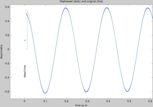
Generated two noiseless Asymmetry plots of same damped signal (5 MHz, 0.3 {$\mu$}s{$^{-1}$}), with different deadtimes (4.2, 5.2 ns), and different phases (15 and 105 deg).
Found phases by auto maxent algorithm. Summed phase-corrected FFT and went back to time domain.
Artifact origin.
Very early times (~ deadtime) are heavily distorted: errors in auto maxent first order phase, proportional to frequency, correspond to a residual small amplitude average deadtime dip. The small additional distortion looks like an exponential with decay ~200 ns starting from t=0.I.e. a Dysonian of width 5 MHz.
|
|
Top.
Prostaferesis
The correct fit function should not produce the value of the Asymmetry fot time equals to the centre of the bin,
rather the integral over a bin of this function. The difference is tiny unless the fucntion is varying very much
within the bin width {$\Delta$}. The integral may be computed exactly (prostaferesis) for harmonic waves with Lorentzian decay, since
{$ A_k= \frac 1 {\Delta} \int_{t_k-\Delta/2}^{t_k+\Delta/2} dt A {\cal Re} \left[e^{i\omega t-\lambda t}\right]={\cal Re}\left[ e^{(i\omega -\lambda) t_k} \, \frac{e^{(i\omega-\lambda) \Delta/2} - e^{-(i\omega-\lambda) \Delta/2}}{(i\omega -\lambda)\Delta} \right]$}
However the computed difference is very small even for frequencies close to the digital passband {$\omega_M=\pi/\Delta t$}, being of the order of 2 10-3. This calculation was implemented in old Muzen but it is not in Mulab.
Top
MORE on GPS
In order to fit results with MORE on GPS (the kicker that diverts incoming muons after a good muon
is implanted) select Toggle mode, now: NO MORE in the setup drop-down. If you look at setup
after that you will see 'Toggle mode, now: MORE''
Remember to go back to NO MORE when switching out of that mode.
A note on MORE: one has to load the corresponding beam solution on the COMBI interface
and to choose an appropriate TDC setting, e.g. 2 ns over 20 us. Be aware that
- the maximum rate is 25000 events/s
- the initial 3-400 ns still have a background, and not a constant one.
- the minimum resolvable relaxation rate is of order 0.02 us-1
Top
rehash after adding new functions
When adding new functions to toolbox/local/mulab-1.05/run a new instance of matlab and issue rehash toolbox to force rereading the toolbox
Top
Linear relations (and shared parameters) in Ver.2.0
Typical use is in the new Double fit of two pairs of detectors at a time, e.g. for the model damu
 UD/FB   1 0.93 ~                       DePhi   2 90 ~
 dalpha  3 0.01 ~      4 ~              muAmp   5 0.13 ~  6 =p(1)*p(5)
                                        muGau   7 750  ~  8 =p(7)
                                        muPhi   9  10  ~ 10 =p(9)+p(2)
 muAmp  15 0.08 ~     16 =p(1)*p(15)    muDeLo 11   0. ! 12 =p(11)
 muGau  17 760  ~     18 =p(17)         muDeGa 13  1.5 ~ 14 =p(13)
 muPhi  19  10  =p(9) 20 =p(9)+p(2)
 muDeLo 21  0.2 ~     22 =p(21)
 muDeGa 23  0   !     24 =p(23)
This scheme will fit a damumu model with 24 nominal parameters, but only 11 independent parameters for the two pairs:
- independent dalpha parameters for the two independent AlphaFB and AlphaUD values
- linked amplitudes between FB and UD within each mu component
- equal fields within each mu component
- equal phases between the two components, and phase shifted by about 90 degrees between FB and UD pairs
- equal Gaussian decay rate in the first mu component
- equal Lorentzian decay rate in the second mu component
Top
< mulab main tools | Index | The internal structure of mulab: Globals >