• View
• Edit
• History
• Print

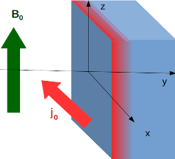
LondonModel

< Superconductors | Index | Pippard corrections: clean vs. dirty superconductors >

From the viewpoint of Maxwell equations a superconductor is characterized by the magnetic flux expulsion, the Meissner-Ochsenfeld effect, which encompasses the whole magnetic behaviour of type I superconductors. A cylindrical specimen of such a superconductor becomes a normal conductor above a critical field {$H_c$} and expels the magnetic flux below {$H_c$}.

Type II superconductors give rise to the same effect below a first critical field {$H_{c1}$}, although they have a more complex behaviour above (the already mentioned Abrikosov lattice). For an extensive description of superconductivity refer e.g. to Tinkham.

Here we show the constraints that Maxwell equations impose on this expulsion, leading to a finite length {$\lambda$}, required by supercurrents to shield the applied field. The essential of this derivation is due to Heinz and Fritz London. The views of Fritz London on superconductivity were essential for the subsequent explanation by Bardeen, Cooper and Schrieffer, and also instrumental for a new, correct approach to the old issue of measure in quantum mechanics.

Maxwell equation (stationary, no charges) read:

{$ (1) \qquad\qquad \begin{eqnarray} \nabla\cdot \mathbf{ E}&=&0 &\qquad\qquad\qquad\qquad& \nabla\times\mathbf{ E}&=& 0&\\ \nabla\cdot\mathbf{B}&=&0 &\qquad\qquad\qquad\qquad& \nabla\times\mathbf{B}&=& \mu_0&\mathbf{j} \end{eqnarray}$}

and the electric field vanishes. Introducing the vector potential {$\mathbf{B}=\nabla\times\mathbf{A}$} only the last equation is non-trivial, namely

{$ (2) \qquad\qquad \nabla\times\nabla\times\mathbf{ A}=\mu_0\mathbf{j}.$}

The identity {$\nabla\times\nabla\times \mathbf{ A}=\nabla(\nabla\cdot\mathbf{ A})-\nabla^2\mathbf{ A}$} suggests the choice of the Coulomb gauge ({$\nabla\cdot\mathbf{ A}=0$}).

The simplest geometry is that of an infinite superconducting semispace to the right, {$y>0$}, with an external induction field {$B_0\hat z$} from sources on the left. It is easy to see that the solution to this problem is a supercurrent density

{$$\mathbf{j}(\mathbf{r})=-j_0 e^{- y /\lambda}\hat x$$} for {$y>0$} and zero otherwise, with {$B_0=\mu_0\lambda j_0$}. The Ampere-Maxwell equation is satisfied with {$$\mathbf{B}(\mathbf{r}) = B_0 e^ {-y/ \lambda} \hat z$$} as can be verified straightforwardly by calculating {$$\left| \begin{matrix}\hat{x}&\hat{y}&\hat{z}\\ \partial_x&\partial_y & \partial_z \\ 0 & 0&B_0e^{-y/\lambda}\end{matrix}\right|$$} This represents a surface current density decaying over a length {$\lambda$}, producing a surface magnetic field with the same penetration length.

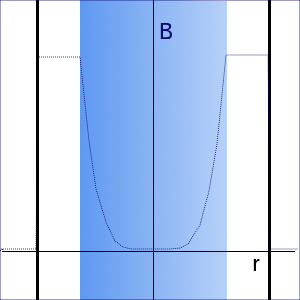
Another simple geometry is that of a superconducting cylinder inside an infinite conventional solenoid with parallel axes. In the stationary case, no net charges. Outside the superconductor volume the solution is straightforward. If the conventional solenoid of radius {$R$} has an ideal surface current density {$j(r)=k\delta(r-R)$} circulating in the plane perpendicular to the solenoid axis, {$\hat z$}, the stationary solution is

{$ (3) \qquad\qquad \mu_0 H = \left\{\begin{align*} &0\qquad\qquad\quad \mbox{outside the solenoid} \\ & \\ &\mu_0 k \hat z \qquad\qquad \mbox{inside the solenoid} \end{align*}\right. $}

This equation, the London equation, is obtained assuming that the superconducting state conserves its vanishing quantum expectation value of momentum {$\mathbf p$}, even in a field, when the canonical substitution implies that {$m{\mathbf v} = {\mathbf p} + e{\mathbf A}$}. Therefore {${\mathbf J}=ne\langle {\mathbf v}\rangle = -\frac {ne^2} m {\mathbf A}$}, and the London penetration depth is {$\lambda = \sqrt{\frac {m}{\mu_0 ne^2}}$}.

As a matter of fact, taking the rotor of the last of Maxwell Eqs. 1, ({$\nabla\times(\nabla\times\mathbf{B})=\nabla(\nabla\cdot\mathbf{B}) - \nabla^2\mathbf{B}$}) and applying the quoted identity to the double rotor on the left hand side, inside the superconductor we get

{$ \qquad\qquad -\nabla^2 \mathbf{B} = \mu_0 \nabla\times \mathbf{J_s}, $}

which, by London Eq. 4, becomes

{$ (5) \qquad\qquad \nabla^2 \mathbf{B} = \frac 1 {\lambda^2}{\mathbf B}. $}

It is easy to recognize that the solution of this equation matching the boundary conditions, Eq. 3, is a radial exponential decay of the magnetic field from its boundary value. If we center the cylindrical radial coordinate {$r$} on the superconductor axis and assume a cylinder radius {$r_0$} {$ (6) \qquad\qquad \mathbf{B}(r) = \mu_0 k\, e^{-(r_0-r)/\lambda}\,\hat z $} satisfies both Eqs. 5 and 3. The supercurrents themselves will then be along the tangent unit vector {$\hat t $} according to {$ (7)\qquad\qquad \mathbf{J}_s(r) = \frac k \lambda \, e^{-(r_0-r)/\lambda}\,\hat t $}

Blue dashed line: field profile inside the solenoid (black tube) and the superconductor (blue cylinder)

The value of the penetration depth {$\lambda$} was derived by London assuming that, upon application of an external field {$\mu_0 H$} the superconducting state retains its zero total momentum, the average value of {$\mathbf{p}=m\mathbf{v}+e\mathbf{ A}$}. The classical definition of current density then implies that {$J_s=ne\langle v\rangle= ne (-\,\frac {eA} m)$}, which justifies London Eq. 4 and fixes: {$ (8) \qquad\qquad \lambda= \sqrt{\frac m {\mu_0 n e^2}} $}

< Superconductors | Index | Pippard corrections: clean vs. dirty superconductors >