< Relaxation functions | Index | A Gaussian distribution of Kubo relaxations >
Abragam, Fig. IV 2]]. For a direct µSR improvement of the Kubo-Toyabe function in simple lattices, see also Celio).
The relaxation function that one observes e.g. with nuclear dipolar fields is the static Kubo-Toyabe function, from the name of the two authors who calculated it first. Its Gaussian form is appropriate for fields whose distribution is a Gaussian of standard deviation {$\frac \Delta {2\pi\gamma} $}, centered at zero, {$p_G(B)=\frac {\sqrt{2\pi}}\Delta e^{-\frac 1 2 (2\pi\gamma_\mu B/\Delta)^2}$}. This is roughly[1] the case of a nuclear species dense on a lattice (abundant isotopes).
|
The relaxation function is given by
{$ (1)\qquad \qquad G_G(t)= \frac 1 3 \left[1 +2(1-\Delta^2t^2) e^{-\frac {\Delta^2t^2} 2}\right] $}
and it is worked out in details in a paper by R. Kubo by means of a stochastic model.
In the opposite limit of randomly diluted nuclei on a lattice the Lorentzian field distribution {$p_L(B)=\frac {\gamma_\mu} {\Delta} \,\frac 1 {1+ (2\pi\gamma_\mu B/\Delta)^2}$} is more appropriate (as shown by Walstedt) and the corresponding relaxation function is
{$ (2)\qquad \qquad G_L(t)= \frac 1 3 \left[1 +2(1-\Delta t) e^{-\Delta t} \right] $}
|
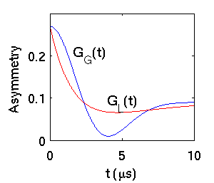
Gaussian and Lorentzian Kubo-Toyabe relaxation, with a typical asymmetry of 0.27.
|
Both functions recover one third of the initial asymmetry at long times, which is due to the longitudinal component of the local fields averaging to an equal fraction of the total field in the distribution. However the Gaussian relaxation shows a marked dip before that recovery, which is the reminder of the overdamped precession around the transverse component of the local field.
The Kubo paper describeas a stochastic treatment of the relaxation function that includes also the effects of the dynamics, represented by a characteristic time {$\tau$} of the time correlations of the local field, and of the external field, {$B_0$}.
Dynamics is taken into account by means of the so-called Markov chain, or strong collision, i.e. collisional events take place such that within the characteristic time {$\tau$} all memory is lost of the previous evolution. For instance this is just the hypothesis behind the relaxation time {$\tau$} in the classical Drude model of metallic conduction.
|
In the case of a strong external field {$B_0$} this model recovers two quite general results for the transverse geometry:
- that in the limit of slow modulation of a stochastic interaction from a Gaussian distribution {$p_G(B)$}, the so called static-limit where {$\omega_0=2\pi\gamma_\mu B_0>\Delta\gg\frac 1 \tau$}, the relaxation function turns out to be
{$ \qquad \qquad(3)\qquad \qquad G(t)= \cos (\omega_0 t +\phi) e^{-\frac {\Delta^2 t^2} 2} $}
where the relaxing term {$e^{-\frac {\Delta^2 t^2} 2}$} is proportional to the Fourier transform of the distribution {$p_G(B)$}, i.e. the lineshape itself reflects the distribution.
|
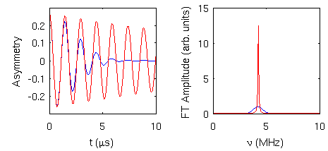
Left: transverse precession with static and motionally narrowed relaxation; right: Fourier transform of the two signals, same color code.
|
- that in the limit of fast modulation, {$\frac 1 \tau\gg\Delta$}, the same Gaussian distribution produces the so-called motional narrowing of the line: the lineshape narrows and the relaxation becomes slower
{$ \qquad \qquad(4)\qquad \qquad G(t)= \cos (\omega_0 t +\phi) e^{-\Delta^2\tau t } $}
where the Fourier transform linewidth is reduced to {$\frac 1 {T_2} = \Delta^2\tau$}. This is typically the result obtained with a nuclear dipolar field when fast muon diffusion has set in, but fast paramagnetic fluctuations in the presence of a local instantaneous hyperfine field produce a similar effect.
|
The static limit in the longitudinal geometry yields a relaxation function which requires numerical methods to be included in a fit routine, The expression derived by Kubo for the Gaussian field distribution is:
{$ \qquad\qquad G(\omega_0,t)= 1 -\left[\frac {\Delta^2} {\omega_0^2}\left(1+\cos\omega_0t e^{-\frac{\Delta^2t^2} 2}\right) -\frac {\Delta^4}{\omega_0^3}\int_0^t \,dx \,\sin\omega_0x\, e^{-\frac{\Delta^2x^2} 2}\right].$}
although a more useful equivalent expression for the numerical calculation is
{$ (5)\qquad\qquad \begin{eqnarray}G(\omega_0,t)= 1 + 2\Delta^2\int_0^t \,xdx \,e^{-\frac{\Delta^2x^2} 2}&\,&\left[\left(\frac {\Delta^2}{\omega_0^2}- 1\right)\,\frac{\sin\omega_0x}{\omega_0x}\right. \\ &-& \left. \frac {\Delta^2}{\omega_0^2} \,\cos \omega_0 x \right]\end{eqnarray}.$}
|
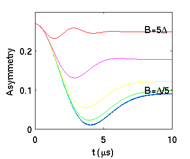
The effect of increasing longitudinal fields on the Gaussian Kubo-Toyabe function. The plotted functions are {$AG(t)$}.
|
We quote here the equivalent expression for the Lorentzian field distribution
{$(6)\qquad\qquad G(\omega_0,t)= 1 +\left(\frac{\Delta}{\omega_0}\right)^2 - e^{-\Delta t}\,\frac \Delta{\omega_0} \left[\frac{\Delta}{\omega_0}\frac{\sin \omega_0t}{\omega_0t}+\frac 1{\omega_0t}\left(\frac{\sin \omega_0t}{\omega_0t}-\cos\omega_0t\right) \right]-\Delta \left[1+\left(\frac{\Delta}{\omega_0}\right)^2\right]\int_0^t \,dx \,e^{-\Delta x}\,\frac {\sin\omega_0 x} {\omega_0 x}$}
|
Finally the longitudinal field relaxation can be calculated in the presence of a dynamical process that makes on average a jump after each {$\tau$}, changing to a different value from the same (e.g. Gaussian) distribution {$p_G(B)$}. This is the so-called strong collision limit of a Markoffian process, appropriate for instance for muon diffusion in zero external field. It may be computed following R.Kubo and Hayano, via a simple expansion and its Laplace transform, although with a numerical trick, as it is shown in the figure on the right. The behaviour may be understood as follows:
- for slow jump rates {$\nu<1$} only the long time longitudinal tail is affected (see for instance the purple curve for {$\nu=0.2$})
- for fast jump rates {$\nu>1$} there is motional narrowing of the relaxation process, i.e. it becomes a simple exponential decay, and the slower, the faster the jump rate (see the black curves).
|
Time dependence of the muon polarization; time is scaled by the parameter {$\Delta$} of the static distribution, and so is the jump frequency {$\nu=1/\tau$}
|
An analytical approximation for this expression, valid also in the longitudinal field case, may be found in the paper of A. Keren
< Relaxation functions | Index | A Gaussian distribution of Kubo relaxations >