< The Abrikosov lattice in type II superconductors | Index | The field distribution probed by muons >
We discuss here the crudest London approximation of the Abrikosov lattice. In the single fluxon case of the previous page, Eq. 3, the field distribution is derived from a modified London equation: the proportionality between currents and vector potential assumed by the Londons' Eq. 2 would imply {$\frac {\lambda^2} {\mu_0}\mathbf{\nabla}\times\mathbf{J}_s + \mathbf{B}=0$}, with full flux expulsion from the bulk of the superconductor. For one fluxon in the origin the extension is
{$$ \qquad\qquad \frac {\lambda^2} {\mu_0}\mathbf{\nabla}\times\mathbf{J}_s + \mathbf{B}= \Phi_0 \delta(\mathbf{r})\hat z,$$}
(this can be also derived under crude approximations from the G-L equations). Combined with Maxwell equations {$\mathbf{\nabla}\times\mathbf{B}=\mu_0\mathbf{J}_s$} and {$\mathbf{\nabla}\cdot\mathbf{B}=0$} one gets
{$$ (1) \qquad\qquad \nabla^2\mathbf{B}=\,\frac {\mathbf{B}} {\lambda^2}\, -\, \frac {\Phi_0} A \delta(\mathbf{r})\hat z, $$}
where A is the sample area perpendicular to the field. We have already illustrated the solution of this equation in the picture beside Eq. 3. It is thus immediate to further extend this derivation to the Abrikosov solution, Eq. 1 to get
{$$ (2) \qquad\qquad \nabla^2\mathbf{B}=\,\frac {\mathbf{B}} {\lambda^2}\, -\, \frac {N\Phi_0} {A} \sum_{n,m} \delta(\mathbf{r}-\mathbf{R}_{nm})\hat z, $$}
|
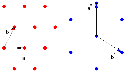
where N is the number and {$\mathbf{R}_{nm}=n\mathbf{ a}+m\mathbf{ b}$} are the coordinates of the flux lattice sites. The solution of this equation was obtained independently by P. Pincus to describe the first NMR experiments, corrected and extended by Barford and Gunn for the first µSR experiments on high-Tc superconductors and, independently, by Brandt. The trick is to solve Eq. 2 in the reciprocal flux lattice, whose unit vectors are
{$$\qquad \qquad \mathbf{ a}^*=\frac {2\mathbf{ b}\times\hat{z}}{ab}\qquad\qquad\mbox{and}\qquad\qquad \mathbf{ b}^*=\frac {2\mathbf{ a}\times\hat{z}}{ab}. $$}
This is done by substituting
{$$\mathbf{B}(\mathbf{r})=\sum_{\mathbf G} \mathbf{B_G} e^{i\mathbf{G}\cdot\mathbf{r}}$$}
with {$\mathbf{G}=h\mathbf{ a}^*+k\mathbf{ b}^*$}, into Eq. 2.
Considering an isotropic superconductor, within the approximation of this treatment, the field inside a unit cell of the flux lattice is given by
{$$ (3)\qquad \qquad B(\mathbf{r}) = \frac {\phi_0} {\mathbf a \cdot b}\, \sum_{h,k} \frac {K_0({ |h \mathbf{ a}^*+k \mathbf{ b}^*|\xi})}{1+\lambda^2\left|h\mathbf{ a}^*+k\mathbf{ b}^*\right|^2}\, e^{i( h\mathbf{ a}^*+k\mathbf{ b}^*) \cdot \mathbf{ r}} $$}
|
Left: a triangular flux lattice, with the unit cell; Right: its reciprocal lattice, with the unit cell
|
|
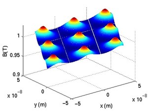
Since the function {$K_0$} acts effectively as a cut-off in reciprocal space it is not difficult to generate the function of Eq. 3 numerically. Of course it is only necessary to generate it inside one unit cell, or less, exploiting its symmetries. The figure on the right shows the result in a two-dimensional cross section perpendicular to the field direction {$\hat z$}.
Neglecting the cut-off the field of Eq. 3 may be viewed as the sum of lattice waves weighted by a Lorentzian of breadth {$\lambda^{-1}$}, which produces an exponentials of decay constant {$\lambda$} centered at each direct lattice site, as it is shown on the right. The cut-off rounds the singularity of the exponential at each site over an area {$\xi^2$}.
|
|
|
By chosing a suitable mesh inside (a portion of) a unit cell one can generate the field distribution, just as the histrogram of the generated field values
This is what is done on the right.
Notice the minimum field, corresponding to the center of the lattice cell, the maximum field, corresponding to a very small area at the center of each core, and the most frequent field value, the peak in the distribution, corresponding to the saddle midpoint between adjacent fluxons.
Note also that {$B_0$}, the average field value inside the superconductor, is equal to {$ {\Phi_0} /({\mathbf a\cdot \mathbf b})$}. This is the first moment of the field distribution (3) and it is reduced by the diamagnetic susceptibility, corrected for demagnetizing effects due to the sample shape.
|
|
< The Abrikosov lattice in type II superconductors | Index | The field distribution probed by muons >