• View
• Edit
• History
• Print

DMu

< FMu | Index | FMu in longitudinal field >

The ²H-Mu system

The difference from the previous case is the addition of a quadrupolar term to the Hamiltonian. As in the purely dipolar case we choose {$\hat z$} along {$\mathbf r$} in order to simplify the dipolar Hamiltonian, If we assume for simplicity a cylindrical electric field gradient along the C-D bond we might have a situation like the one depicted in the figure for a Mu-C-D block. D=2H has spin {$S=1$}; assuming the vector from Mu to 2H along {$z$}, {$\eta=(q_{x'x'}-q_{y'y'})/q_{\zeta\zeta}=0$} for the Electric Field Gradient tensor {$e\mathbf q$}, and a generic orientation of its principal axis {$\zeta$} with respect to {$z$} described by the angle {$\theta$} the Hamiltonian is: {$ \frac {\cal H} \hbar = -\omega_d(2I_zS_z-I_xS_x-I_yS_y) + \frac {\omega_Q} 2 (S_\zeta^2-\frac {S(S+1)} 3) $}

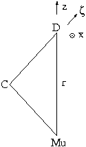
where (see the quadrupolar interaction) {$\omega_Q(\theta)=3\frac{eQ V_{\zeta\zeta}(3\cos^2\theta-1)}{2\hbar S(2S-1)}$} and the matrices for S=1 are

{$ S_x= \frac {\hbar} {\sqrt 2}\left(\begin{array} 0 & 1 & 0 \\ 1 & 0 & 1 \\ 0 & 1 & 0\end{array}\right )\qquad S_y= \frac {\hbar} {\sqrt2} \left(\begin{array} 0 & -i & 0 \\ i & 0 & -i \\ 0 & i & 0\end{array}\right )\qquad S_z= \hbar\left(\begin{array} 1 & 0& 0 \\ 0 & 0 & 0 \\ 0 & 0 & -1 \end{array}\right )$}

The constant term {$I(I+1)/3$} in the Hamiltonian may be dropped to investigate transitions. We consider the tensor product space of I and S, with inner S, i.e.

{$I_z=\frac 1 2 \left(\begin{array}1 & \quad 0 & \quad 0 & \quad 0 & \quad 0 & \quad 0 \\ \quad 0&\quad 1&\quad 0&\quad 0&\quad 0&\quad 0\\ \quad 0 &\quad 0&\quad 1&\quad 0&\quad 0&\quad 0\\ \quad 0&\quad 0&\quad 0&-1&\quad 0&\quad 0\\ \quad 0&\quad 0&\quad 0&\quad 0&-1&\quad 0\\ \quad 0&\quad 0&\quad 0&\quad 0&\quad 0&-1 \end{array}\right )$}

 Hence with the above ingredients one finds

{$\frac {\cal H} \hbar = \left(\begin{array} \omega_d+\frac{\omega_Q} 2(1-\frac{\sin^2\theta}2) & \quad \frac {\omega_Q} {2\sqrt 2}\sin\theta\cos\theta & \frac {\omega_Q} 4 \sin^2\theta & \quad 0\quad & \quad 0\quad & \quad 0\quad \\ \quad \frac {\omega_Q} {2\sqrt 2}\sin\theta\cos\theta & \quad \frac {\omega_Q} 4 \sin^2\theta &\quad \frac {\omega_Q} {2\sqrt 2}\sin\theta\cos\theta & \quad \frac {\sqrt 2} 2 \omega_d & \quad 0\quad & \quad 0 \quad \\ \quad \frac {\omega_Q} 4 \sin^2\theta & \quad \frac {\omega_Q} {2\sqrt 2}\sin\theta\cos\theta & -\omega_d+\frac{\omega_Q} 2(1-\frac{\sin^2\theta}2) & 0 &\quad \frac {\sqrt 2} 2 \omega_d & 0 \\ \quad 0 \quad & \quad \frac {\sqrt 2} 2 \omega_d &\quad 0 \quad & -\omega_d+\frac {\omega_Q} {2}(1-\frac{\sin^2\theta} 2) & \quad \frac {\omega_Q} {2\sqrt 2}\sin\theta\cos\theta & \quad \frac {\omega_Q} {4}\sin^2\theta\\ \quad 0 \quad & \quad 0 \quad & \quad \frac {\sqrt 2} 2 \omega_d & \quad \frac {\omega_Q} {2\sqrt 2}\sin^\theta\cos\theta & \quad \frac {\omega_Q} {4}\sin^2\theta & \quad \frac {\omega_Q} {2\sqrt 2}\sin\theta\cos\theta \\ 0 & 0 & 0 & \quad \frac {\omega_Q} {4}\sin^2\theta & \quad \frac {\omega_Q} {2\sqrt 2}\sin\theta\cos\theta & \omega_d+\frac {\omega_Q} {2}(1-\frac{\sin^2\theta} 2)\end{array}\right )$}

< FMu | Index | FMu in longitudinal field >