< Spin echoes | Index | The spin echo to measure T2 >
Generating a spin echo with matlab
Thus the matlab routine for nutation gives us the essential of a pulse routine. It must take the density matrix at the beginning of the pulse as an input, and provide the same matrix after the nutation induced by the radio frequency field as an output.
The free evolution routine may be built along the same principle. We always keep in the rotating frame, to avoid visualizing very fast and uninteresteng precessions at frequency ω. For this first case of a non interacting spin ensemble, the free evolution of each isochromat is then determined by the simple Hamiltonian, H_0=h(ω0-ω)Iz , via its U and U-1 evolution operators.
The successive application of a second pulse is then the straightforward repetition of the first. Imagining suitable functions rho=pulse(rho,...) and rho=freeevol(rho,...), each fed with appropriate parameters, we can sketch the echo simulation as follows:
rho0=Iz;
rho=pulse(rho0,...);
rho=freevol(rho,tau);
rho=pulse(rho,...);
m=acq(rho)
where the last line implies e.g. the measurement, during free evolution, by means of trace(rho*Iy), for an appropriate time interval following the last pulse.
|
|
It is interesting to track each isochormat independently.
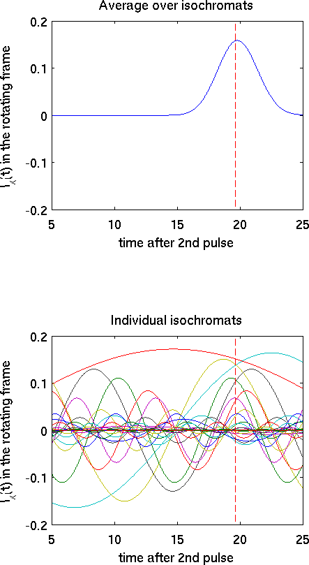
Fig. 1 The sum of all isochromats produces the echo, which means that at a generic time all isochromats are interfering destructively with one another and only around time τ after the center of the second pulse they interact constructively. In this numerical simulation, as in the case of simple nutation, we set h=1 and ω_1=0. A Gaussian envelope was chosen for the isochromats, with standard deviation equal to 1 (i.e. equal to ω_1). Notice the positive sign of the echo, along {Ł \hat {y'} Ł}. The amplitude is also reduced (in the same simulation the maximum FID amplitude is equal to {Ł 1/\sqrt {2\pi} \approx 0.4 Ł}).
|
|
|
|
|
Fig. 2 The different colours represent the contributions of each isochromat with weights according to the Gaussian envelope. The destructive interference is readyly visible: at times where the lines of different colors are equally distributed above and below zero their sum must be vanishing. By the same principle the constructive interference can be spotted, The verical line marks the position which corresponds to time t=τ+tw/2'
|
< Spin echoes | Index | The spin echo to measure T2 >