• View
• Edit
• History
• Print

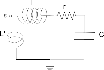
Probehead

< Block diagram of an NMR experiment | Index | Resistive probeheads >

The simplest probe-head operates at room temperature and is built around a variable capacitor in air to make a resonating circuit at variable frequency, with high {$Q=\omega L/r$} factor so that a rather large current circulates in the coil, producing a large radio-frequency field to nutate the nuclei in a short time. This means small series resistance {$r$} in the probe. However a pure rLC circuit would have impedance {$r$} at resonance. Such a small impedence would lead to the reflection of most of the power incoming from the transmitter, with only a minute fraction going actually through the coil.

In order to get power through the coil one has to degrade a bit the resonance and produce a total input impedence of the probe equal to that of the lines ({$Z_0=50 \Omega$}), i.e. to the output impedence of the transmitter and to the input impedence of the receiver. This is described as matching the impedence to {$Z_0$}, while tuning the probe to the desired frequency.

The circuit shown in the figure is a simple one that allows simultaneous matching and tuning. The pure series rLC could be tuned to resonance by varying the capacitance, but this would produce a total input impedence equal to the resistance r, which is kept very small to obtain a large merit factor (this results in a corresponding amplification of the current through the inductance, i.e. of the radio-frequency field {$B_1$}. The circuit in the figure can be tuned slightly out of resonance, to produce a capacitor-like imaginary impedence from the series. This can be compensated by the parallel additional inductance to leave an amplified total real impedence that can be matched to 50 Ohm (the characteristic impedence of the line as well as the transmitter output impedance).

Fig. 1

Work out how this may be done by calculating the circuit equations.

Top

Another useful simple circuit is shown in the figure and we sketch the solution for this one. Let's first calculate the right side of the transformer, assuming that the currents circulating in the primary (left) and in the secondary (right) winding are out of phase. This may happen only if the transformer is not ideal, but we may disregard the details and just assume a net phase {$\phi_0$} for the current {$I_0$} circulating on the left. {$0=i\omega M I_0 e^{i\phi_0}+\left[i\left(\omega L- \frac 1 {\omega C}\right) + r\right] I_1$} Normalizing to {$I_0$} the current amplitude ratio {$i_1=I_1/I_0$} is readily obtained as {$ (1) \quad\quad i_1= \frac {\omega M}{\left| \omega L - \frac 1 {\omega C} \right|}\approx \frac{\omega_0 M^2}{2L\Delta \omega}$}

Fig. 2

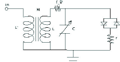
where {$\omega=\omega_0 + \Delta \omega$} is slightly shifted from the resonance frequency {$\omega_0=1/\sqrt{LC}$} (and still {$\left| \omega L - \frac 1 {\omega C} \right|\gg r$}). Also the phase may be obtained as

{$ (1) \quad\quad \tan \phi_0 = \frac {\omega M}{\left| \omega L -\frac 1 {\omega C}\right|}\approx \frac r {2 L \Delta \omega}$}

We can now look at the left side of the transformer. Here we want the input impedence to be real and equal to {$Z_0=50 \Omega$}, hence the current {$I_0$} must be in phase with that of the transmitter. Therefore here we will attribute the phase difference, {$\phi_1=-\phi_0$}, to the current of the secondary winding and write

{$Z_0=i \omega L^' I_0 + i \omega M I_1 e^{-\phi_0}$}

which corresponds to {$Z_0=\omega M i_1 \sin\phi_0$} and {$L^'=-i_1 M \cos\phi_0$}. This implies that {$\pi/2<\phi_0<\pi$}, so that the sine is positive and the cosine is negative, i.e. we need a shift {$\Delta\omega<0$}. Substituting Eqs. (1) and (2) into these expressions, and recalling that r is much smaller than all other impedances in the circuit, we obtain

{$ (3) \quad\quad \frac{Z_0} r \approx \left(\frac {M}{2L} \frac {\omega_0}{\Delta \omega}\right)^2; \quad \quad \quad (4) \quad\quad M\approx \sqrt{2LL^' \frac{\left|\Delta \omega\right|}{\omega_0}$}

Summarizing, by tuning the variable capacitor to a slightly larger value ({$\Delta\omega<0$}) and the mutual inductance {$M$}, we can satisfy at once Eq. 3 to match the real {$Z_0$} value of the cable and Eq. 4 to guarantee no imaginary impedence.

Top

What to do when the required power is too low?

If we try to transmit a pulse of lower amplitude than required to polarize the diode bridge the pulse will not get through. We need a trick. We may transmit a pulse of larger amplitude and selectively degrade the Q of an appropriate amount the probe upon transmission, recovering the full Q upon detection. This is achieved by another diode bridge inside the probe, by modifying the two former circuits of Fig. 1, 2.

Fig. 3: RLC with diodes (A is the hot point where {$V=QV_{in}$})

Fig. 4: Transformer LC with diodes

For the low detection level of the NMR signal the added diodes do not conduct, hence the circuit has the same Q as in Fig. 2. For the higher transmission level of the pulses the diodes are in conduction and the parallel resistance (typically tens or hundreds of kΩ) reduces the Q of the LC circuit.

Important!, remember to tune the probe in very low power conditions ({$V_{in}<V_{diodes}/Q$}) since that high Q condition will have the narrowest bandwidth. The probe is tuned over a wider band in transmission, when Q is degrated. Check that there is a change in bandwidth with excitation dbm, by sweeping the frequency in the tuning setup.

Top

< Block diagram of an NMR experiment | Index | Resistive probeheads >