
|
Chapters:
|
MuSR /
MulabPrimer< Mulab: a matlab toolbox shareware | Index | mulab main tools > Mulab is easy Tested under linux and Windows (XP, Vista, 7). Before you start: Reference manual Some reference help is always available with the matlab scheme ( The most informative are (type them in lowercase from command prompt, as usual in matlab): HELP MULAB, skeleton directives HELP MUFIT_GUI, the reference for the main Menu window HELP MULAB-x.xx/CONTENTS (e.g. MULAB-1.05), the synopsis of the routines You must first chose in advance your logging policy, see Mulab Data Logs for details You have a directory with data files, and the filenames have a specific prefix and suffix. The former is the filename part before the run number, the latter is data-format specific. Mulab must be told of both.
It is suggested that you work (i.e. launch matlab) in a facility and instrument specific directory, where you save a MULAB.mat startup file specific for that setup, e.g. /home/user/mulab/psi/gps/ so that you do not have to deal with these issues more than once.
Mulab will then know three directory paths, that of the data (stored in MU_PATH.DATA, i.e. field DATA of global structure MU_PATH), the working directory, (MU_PATH.ROOTDIR) and that for the logs (MU_PATH.LOG).
Create the instrument-specific directory. You can now launch matlab from it. For instance under Windows you can duplicate the Matlab link on the Desktop, rename it to e.g. Mulab_gps, edit its properties and copy the instrument-specific path into the From input box. Under linux you simply cd to the directory and invoke Now make sure that matlab knowns mulab, i.e. that the mathlabpath contains the toolbox: Under windows click the File/Set Path.. menu, press Add, select the toolbox/local/matlab-x.xx directory, then press Save and Close.
Under linux insert a line
addpath('/usr/local/matlab/toolbox/local/mulab-x.xx')
in your To check that this works, type Inside matlab: initial settings Now type mulab from the command line. If you have no MULAB.mat yet, answer y to Proceed [N] and then answer to a set of simple questions: Facility (PSI, ISIS), Instrument(GPS, DOLLY, LTF, MUS, EMU, HIF), Data Format (ASCII, BIN, MCS, NEXUS), File prefix (write the case sensitive, initial part of your file names, before the run number), file suffix (the extension), A Menu window (Graphical User Iinterface, GUI) should appear. You should see a picture like this (not quite, you do not have parameters set and data loaded) 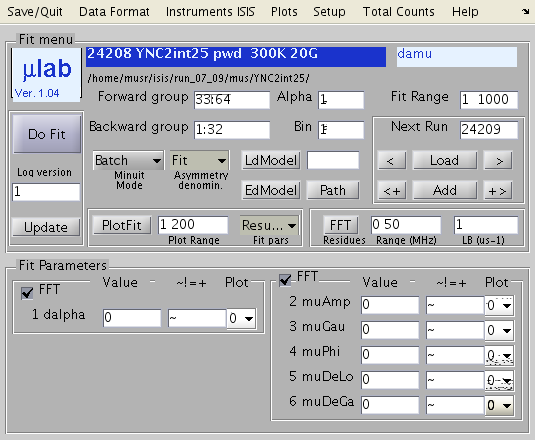 First thing, look at the Save/Quit dropdowns and select LOCATION
FILENAME PREFIX
LOG PATH policy
according to the choice that suits you (see Mulab Data Logs for details). Hopefully your answers set this right already. Then make sure you have the right data path: press the PATH button. If you have chosen Log Path Selectable at home, you will also be prompted to choose the log dir. Then load a data set: press Load. Now you can calibrate where t=0 falls within your time bins. For a rough guess simply go to the Menubar, drop down Setup and choose Determine t=0. The right way is to run field dependent experiments, correct for field dependent initial precession (at PSI with spin rotator ON) and fix by hand. Keep in mind that t0 is an integer equal to the bin containing time t=0
-0.5<dt<0.5 is the fine tuning of t=0 within that bin
offest is an integer equal to the number of bins between t0 and the first good (or usable) bin.
When the first number in Fit Range is 1, analysis (fit and FFT) starts from bin t0+offset. See Setup below for furthe details. Fit models: the name of the game Fits are performed over asymmetries, after selection of a Forward group of detectors (say detector 3 in gps) and a Backward group (say 4 in gps). If you must select more complex patter, like Up-Down on MUSR, follow this syntax Forward group: 1:5 32:39 64
Backward group: 16:25 47:55
Just write these space and colon separated numbers in the two edit windows (for WIN purposes "=" is a synonym of ":"). If you want to save this group with a name, Menubar Setup-> Save group. You can the Load group as well Calibrate {$\alpha$} (see below) writing its value in the Alpha edit Range is in bins, typically 1 7800 at PSI, 1 1000 at ISIS, starting from the first good bin (you can fine tune it by the offset - see in the Setup dropdown menu, below). Fit models are defined by their names. They are any combination of standard ingredients (with sense), called by a two letter code name. You can make your own, For the time being only the following set is available. da: for dalpha, linear correction for a slightly wrong {$\alpha$} (see its definition, the fit result should be subtracted from the Alpha edit value, and a couple of iterations will yield the correct value of {$\alpha$}, within experimental uncertainty).
ba: for background, a decay, typically a longitudinal fraction or a slowly relaxing muon fraction with nearly vanishing static internal field. It can be Lorentzian and Gaussian. Here and in following cases, in order to have only one type of relaxation rate, fix the other to zero. Parameters are: Asymmetry (baAmp) and Decay Rates (baDeLo and baDeGa) in µs-1.
mu: for muon, a harmonic wave, with Gaussian and Lorentzian relaxation. Precessions in internal oir external fields. Parameters: Asymmetry (muAmp), Field (muGau) in Gauss, Phase (muPhi) in degrees, Decay Rates (muDeGa and muDeLo) in μs-1.
bj: for Bessel J0, representing asymmetries in single q spin density waves. Parameters: same as for mu (bjAmp, bjGau, bjPhi, bjDeLo, bjDeGa).
st: for strecthed harmonic wave. Parameters: stAmp, StGau, stPhi as for mu, plus Relaxation Rate (stDel) )and an exponent (stBeta). stDel varies between 10-3 and 103 μs-1, stBeta between the same numeric values.
kg: for Gaussian Kubo-Toyabe static component, with or without external field. Parameters: Asymmetry (kgAmp), longitudinal Field (kgGau) in Gauss, Gaussian width of the static field distribution (kgDeG), in µs-1, 1/T1 decay (kgDeLo), in µs-1. The last is an independent T1 process. The Gaussian width can only vary between 10-3 and 103 μs-1
kl: for Lorentzian Kubo-Toyabe static component, with or without external field. Parameters: Asymmetry (klAmp), longitudinal Field (klGau), in Gauss, Lorentzian static width of the static field distribution (klDeL), in µs-1, 1/T1 decay (klDeLo), in µs-1. The last is an independent T1 process. The Lorentzian width can only vary between 10-3 and 103 μs-1
mt: for muonium triplet, the two precessing components corresponding to low field triplet muonium transition. See this reference for THE definition of the frequencies. Parameters: Asymmetry (mtAmp, sum of the two), Hyperfine frequency, {$\nu$} (mtHyp), in MHz (4400 for muonium in vacuum), Field (mtGau) in Gauss, Phase (mtPhi) in deg, plus two pairs of relaxation rates, mtDeLo, mtDeGa, mtDeLo, mtDeGa, in μs-1, for the low and high frequency components, respectively.
fl: for flux lattice, the precession pattern expected from the field distribution in the isotropic Abrikosov lattice in the London approximation. To see all details have a look at the function mufll.m. Calculates the spatial field distribution, makes a histogram over field bins worked out from the FFT frequencies of the required time domain. Convoluted with a generic Gaussian broadening. Parameters: Asymmetry (flAmp), internal field (flGau), in Gauss, positive defined and limited to 10 T, Phase (flPhi) in deg, London depth {$\lambda$} (flLmbd), in nm, coherence length {$\xi$} (flXi), in nm, Gaussian width (flDeGa), in μs-1. Strong doubts on the strong correlations among {$ B, \lambda, \xi$}.
fm: for FMuF, the dipolar interaction of three spin 1/2 moments in a linear unit, in zero external field. Parameters: Asymmetry (fmAmp), dipolar field (fmGau), in Gauss, Lorentzian decay (fmDeLo) and Gaussian decay (fmDeGa), in μs-1.
So the model Assume it is a transverse field calibration with 20G. You have already the right fit model (damu) loaded by default. Just put sensible numbers in the parameter edits, where you see zeros now, for the starting guess, say 0.2 for parameter 2, muAmp, 20 for parameter 3, muGau. The input window next to each parameter value is for a symbol representing, respectively ~ for variable
! for fixed
=5 for share the value of parameter 5
+2*p(1)-0.3 for a linear relation forcing this parameter to take twice the value of parameter 1 minus 0.3
So, for instance, put ! in the input next to parameter 6, muDEGa (Gaussian rate), and leave free only the Lorentzian rate, 5 muDeLo (mu and ba components can have either Gaussian or Lorentzian rates or both). Now press PlotFit if you want to display your starting guess. Otherwise you can jus press Do Fit. Have a look at the command window to see the MINUIT printout and the final summary. You will see that the additional parameter da has a best fit value different form zero. This is the first order approximation to a correction term, which you must SUBTRACT from alpha to obtain a better value. Iterate this fit-and- correct scheme a couple of times until da is zero within error. If everything looks fine this is maybe the moment to save your MULAB.mat by pressing MenuBar Save/Quit-> Save Mulab. This will store the present Data and Log Paths, plus filename and location, t0 and offset. Next time you start Mulab these values will be already set. The output appears in the command window: the full MINUIT output, plus a readable summary. Results are stored thrice (and what I tell you three time is true![1]). All under path This is a -mat file, which you can load with A plain ASCII copy of the command window summary is kept in Furthermore one ASCII line per fit, listing pairs of parameter best fit values and their errors, are kept updated in in the order they are given to fminuit. It is essentially the order of the FIT parameter Menu, but shared parameters (=) and those fixed by liner relations (+) are missed out. Three numbers open each line, the run number, the temperture and the field from the title. One can upload these ASCII files in Origin or similar The tag you write in the edit below the Do Fit button is the log version. If you want to refine the present fit and overwrite the log, just go ahead. If you want to perform a new scan of data sets, with a modification within the same model - say from Gaussian to Lorentzian rates, or change share to independent phases in two oscillating components - and you want to keep them both, change version to 2. If you performed several equivalent fits (e.g. of type bamumu) of a large dataset, say a T scan, you now want to plot the results versus T. That is what the popup menus on the right of the parameters are for. If you leave a parameter popup menu flag to 0 it will not appear in the plot. Flags run form 1 to 4, so the plot can have up to four panels. In this way you can group, e.g., asymmetries in panel 1, by selecting 1 in their popup menus, and likewise Relaxation rates in panel 2. Now go to MenuBar-> Plots-> Plot Parameters vs. T. Et voilŕ!. Mulab searches the log directory for all the files whose name matches: the fit model (e.g. bamumu)
the chosen groups (e.g. 3-4)
the present version (e.g. 1)
So you can go back to an old analysis, select the correct log path, load one of the fit models, select the popup flags (if they are not already set) and plot You can also plot vs. nominal field (from title), vs. run number of vs. a user defined variable, x, which you must define from the command line, by typing first global MU_FIG MU_FIG.X=[130 20 43 50:20:110 ... ]; Make sure to define as many values as the number of runs to plot. Then select MenuBar-> Plots-> Plot Parameters vs. x MU_FIG.X=[130 NaN 43 50:20:110 ... ]; And you can still work directly on your data from the command window. Raw data are kept in
the global structure >> global MU_DATA
>> MU_DATA
>> MU_DATA.DATA(300:400,1:4)
at the matlab prompt to see. After a fit the time, asymmetry and asymmetry statistical errors are kept in MU_DATA.TIME, MU_DATA.ASYMMETRY and MU_DATA.ASYMMERRORS, respectively. Innards
Mulab stores global variables in structures, Try also typing at the matlab prompt. References [1] - The Bellman's rule of three. Lewis Carrol. The Hunting of the Snark. ISBN0393062422. < Mulab: a matlab toolbox shareware | Index | mulab main tools > |