|
Chapters:
|
MuSR /
Interactions< Muon sites | Index | Paramagnetic species > The semi-classical muon is a point-like particle. At each interstitial site the muon spin {$I=\frac 1 2$} is subject to interactions with the other spins, those of neighbouring electrons and nuclei. A classification of these interactions similar to that of NMR may be performed, with the simplifying condition that the muon itself, being spin one-half, does not possess an electric quadrupole moment. Hence the muon does not couple to the electric field gradient, although it definitely may produce one. Please note that in these notes we use consistently (?!) the SI units. Assume the muon in the origin of the reference frame, at {$r=0$}, and that a uniform external magnetic field {$B$} is aligned along z.In frequency units the magnetic Hamiltonian is: {$$ \begin{eqnarray}\frac{\cal H} h = \frac 1 h({\cal H}_Z+{\cal H}_{e\mu}+ {\cal H}_{n\mu}) &=& \frac 1 {2\pi} \,\left\{ \,\left[-\gamma_\mu I_z + \gamma_e\sum_{i=1}^{n_e} s_{iz} - \sum_{k=1}^{n_n} \gamma_k I_{kz}\right] B \right.\nonumber \\ &&+\gamma_\mu \mathbf{ I }\cdot \sum_{i=1}^{n_e}\frac {\mu_0}{4\pi} \hbar\gamma_e \left[\frac {{\mathbf l}_i }{r_i^3}+\frac {- \mathbf s_i + 3\hat r_i \,\mathbf s_i\cdot\hat r_i}{r_i^3} + \frac {8\pi} 3 \mathbf s_i \delta(\mathbf r_i)\right] \nonumber \\&& \left.+\gamma_\mu \mathbf I\cdot\sum_{k=1}^{n_n} \frac {\mu_0}{4\pi} \hbar\gamma_k \frac {- \mathbf I_k + 3\hat r_k\,\mathbf I_k\cdot\hat r_k}{r_k^3} \right\}\end{eqnarray}$$} The first row contains the Zeeman interactions, {${\cal H}_Z$} of all the involved spins, {$s_i$} for the {$i$}-th electron and {$I_k$} for the {$k$}-th nucleus, while the second row contain the magnetic interactions between the muon and the electrons, {${\cal H}_{e\mu}$}, and the third those beteen the muon and the nuclei, {${\cal H}_{n\mu}$}. The sum over {$k$} in the last row of Eq. 1, where {$\mathbf r_k=r_k\,\hat r_k$} is the position of the {$k$}-th nucleus, may be recognized as the classical dipolar field, {$\mathbf B_d $}, from nuclear point dipoles, each contributing with {$$ \begin{equation}\mathbf B_{kd} = \frac {\mu_0}{4\pi} \hbar\gamma_k \frac {- \mathbf I_k + 3\hat r_k\,\mathbf I_k\cdot\hat r_k}{r_k^3}\end{equation}$$} The nuclear coordinates may always be treated classically.
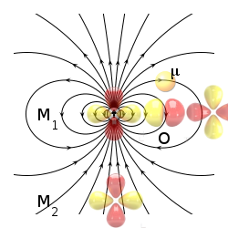
In all these three electron terms the coordinates must be considered as electron operators. Since the electron dynamics is much faster than the muon spin precessions these operators may be averaged over the electron wave functions, recovering a spin-only Hamiltonian. Often the orbital term is neglected because of the quenching of orbital momentum? by crystalline fields (make sure that this is the case!). The second term accounts for the distant magnetic ions, yielding a purely dipolar field by Eq. (3). Electrons involved in the muon chemical bond will contribute via the second and third terms to the so-called hyperfine coupling. This may happen directly, if an unpaired electron of spin {$\mathbf s$} is involved in the bond. Then, assuming that {$z$} is the quantization axis, the second term gives rise to the pseudo-dipolar hyperfine tensor and the third term gives rise to the Fermi contact hyperfine (scalar) coupling: {$$\begin{equation} (\delta\tilde \nu+ \nu_0) I_z= \frac {\mu_0}{4\pi} \frac {\gamma_\mu} {2\pi} \mathbf I\cdot\hbar\gamma_e \left[\langle\Psi| \frac {- \mathbf s_i + 3\hat r_i\,\mathbf s_i\cdot\hat r_i}{r_i^3}|\Psi\rangle + \mathbf s\frac {8\pi} 3 |\Psi(0)|^2\right], \end{equation}$$} respectively the first and second term in parethesis. This is the case when a radical is formed. In inorganic magnetic materials the muon is often bound to an anion (oxygen, fluorine, etc..), which is non magnetic, i.e. the bond is formed, in first approximation, only by paired electrons. A contact and a pseudo-dipolar term may still arise, e.g. a second nearest neighbour magnetic cation, M, may spin polarize the Mu bond, say M-O-Mu, giving rise to a net spin density at the muon. This is the so-called super-hyperfine coupling. Averaging over the intervening electrons, the second and third terms act as a (tensorial) coupling: {$$\begin{equation} (\delta\tilde \nu+ \nu_0 )I_z= \frac {\gamma_\mu}{2\pi} \mathbf I\cdot\left[\delta\tilde A + A_0 \right]\cdot \mathbf S, \end{equation}$$} formally equivalent to those of Eq. (4), although here {$\mathbf S$} may be a composite spin, like that of the ground state of a magnetic cation. A muon however is not a point particle. Let us consider in first approximation the Coulomb potential acting on the muon, that can be approximated e.g. as the total energy {$E(\mathbf r)$} of a DFT calculation with a hydrogen atom at {$\mathbf r$} in the lattice. This is true assuming that the Born Oppenheimer approximation holds for the electrons and the muon. The Schroedinger equation of the muon is then {$$ \left[- \frac {\hbar^2\nabla^2}{2m} + E(\mathbf r)\right]h_j(\mathbf r) = \epsilon_j\, h_j(\mathbf r)$$} It coincides with an oscillator problem, more or less harmonic, depending on the shape of the potential {$E(\mathbf r)$}. Due to the low muon mass {$m$} the zero point energy of the muon, {$\epsilon_0$}, is generally large. The extent of the wave function {$h_0(\mathbf r)$} is determined by the potential. In particular {$\epsilon_0$} may not exist, if the barrier, defined by {$E(\mathbf r)$}, isn't large enough. The local field at the quantum muon must then coincide with the average {$$ \langle \mathbf B_\mu \rangle = \int d \mathbf r |h_0\mathbf r)|^2 \mathbf B_\mu(\mathbf r)$$} where the local field operator {$\mathbf B_\mu(\mathbf r)$} is defined as {$$ \hbar \gamma_\mu \mathbf B_\mu(\mathbf r)\cdot \mathbf I = -\hbar\gamma_\mu B I_z + {\cal H}_{e\mu} + {\cal H}_{n\mu}$$} Let's consider the case of zero external field and, when magnetic order is present, neglect the nuclear interactions. The average local field will then be {$$\langle \mathbf B_\mu \rangle \cdot I = \frac {2\pi}{\gamma_\mu}\int d \mathbf r |h_0\mathbf r)|^2 (\delta\tilde \nu+ \nu_0)$$} < Muon sites | Index | Paramagnetic species > |