|
In a high magnetic field the free electron Hamiltonian becomes
{$$\begin{equation}{\cal H} = \frac 1 {2m} [(\mathbf p + e\mathbf A)^2 + e\hbar \boldsymbol \sigma\cdot \mathbf B]\end{equation}$$}
where we have included the minimal substitution in the first term plus the usual Zeeman term. Let's start by choosing the Landau gauge, {$\mathbf A = \frac 1 2 (-By,Bx,0)$}, so that only {$p_z=\hbar k_z$} is commuting with {$\cal H$} but {$p_x,p_y$} are not. The two components of the linear momentum in the presence of the perpendicular field are {$\pi_x=p_x+eA_x=p_x-eBy/2$} and {$\pi_y=p_y+eA_y=p_y+eBx/2$}, and with the help of the standard commutation relations {$[\alpha,p_\alpha]=i\hbar,\,\alpha=x,y$} we obtain their commutator
{$$[\pi_x,\pi_y]=eB\frac\hbar i$$}
Let us now define a magnetic length {$l=\sqrt{\hbar/eB}$} and the two components of the linear momentum in the presence of the field as (beware, UR has a mistake here)
{$$\pi_x= \frac \hbar {\sqrt2l}(a-a^\dagger)\qquad \pi_x=\frac \hbar {i\sqrt2l}(a+a^\dagger)$$}
The two new operators are therefore {$a=l/\sqrt2\hbar(\pi_x+i\pi_y)$} and {$a^\dagger=l/\sqrt2\hbar(-\pi_x+i\pi_x)$}, and their commutator is
{$$[a,a^\dagger]=\frac 1 {2eB} \frac i {\hbar} [\pi_x,\pi_y] + \frac 1 {2eB}\frac 1{i\hbar} [\pi_y,\pi_x] = \frac i {2eB}\frac 2 {\hbar} \frac {\hbar eB} i =1$$}
Recalling that {$\omega_c=eB/m$} is the cyclotron frequency and that {$\hbar\omega_c/2=\mu_B B$}, with the help of this last commutator we get
{$${\cal H}-\frac {\hbar^2k_z^2}{2m} - \frac {\hbar\omega_c} 2\sigma_z = \frac {\hbar\omega_c} 4 [(a+a^\dagger)^2-(a-a^\dagger)^2]=\hbar\omega_c\left(\hat n+\frac 1 2\right)$$}
The energy levels of this Hamiltonian
{$$\begin{equation}\epsilon_{n,k_z,\sigma} = \hbar \omega_c \left[\left(n+\frac 1 2\right)+\frac {\sigma_z} 2\right] + \frac {\hbar^2 k_z^2}{2m}\end{equation}$$}
are labelled by quantum numbers {$n,k_z,\sigma_z$}. The first resembles a quantum oscillator and representing quantized cyclotron orbits of increasing energy, starting from a finite zero point energy {$\hbar\omega_z/2$}. The second represents standard wave vectors along the field direction, whose number is given by periodic boundary conditions as {$L_z/a$} where {$a$} is the lattice spacing and {$L_z$} the sample length in the field direction. The third is simply the spin direction, {$\sigma=\pm1$}.
Figure 1 shows representative slices of the energy of Eq. (2), supposing that electrons keep their bare mass and g factor in the gas. If we replace these quantities by their effective values {$m^*, g^*$} in the metal, the factor in front of {$(n+1/2)$} and that of that multiplying {$\sigma_z$} in the Zeeman energy become different, the former becoming {$\omega_c=eB/m^*$} and the latter {$g^*\mu_B/2$}
|
 Figure 1. Landau levels vs. field and vs. {$k_z,\sigma_z$}, assuming free electron mass and g-factor. In this condition {$g\mu_B = \hbar\omega_c$} and spin up {$n$} coincide with spin down {$n+1$} bands. The central panel is {$n$} energy levels vs. magnetic field at {$k_z=0$}; the vertical dashed lines indicate two field values and at each of these the left and right panel show the {$k_z$} bands. The dotted horizontal lines show the cyclotron resonance bottom and the gray lines the maximum filling of each band before the next band starts being filled at {k_z=0$}. The maximum number of filled states is the number of electrons divided by 2 (spin), which sets the Fermi energy at {$T=0$}. In both panels {$k_z$} bands overlap (low fields); at high enough fields (the quantum limit) all available states in a band are filled before the next one is reached, i.e. all electrons are in the lowest {$n=0$} band.
|
|
Index
Density of states
The same calculation may be done in this other form of Landau gauge, {$\mathbf A = (0,Bx,0)$}, where also {$p_y=\hbar k_y$} is a good quantum number. Now the Hamiltonian (1) reads
{$${\cal H}=\frac {p_x^2} {2m} + \frac {(eB)^2} {2m} (x-x_0)^2 + \frac {\hbar^2 k^2_z} {2m} + \frac {\hbar \omega_c} 2 \sigma_z$$}
where we have defined(*) {$x_0=-\hbar k_y/eB= l^2k_y$}. The first two term are identical to a harmonic oscillator for each {$k_y$} state, with center of mass {$x_0$}, the cyclotron resonance center. The eigenvectors remain those of Eq. (2). Applying periodic boundary conditions we write {$k_y=n_y2\pi/ L_y$}. Note that in this case the smallest finite value of {$k_y$} is set by field and not by the lattice spacing, and each value of the wave vector has its own (absolute value of) center of mass {$x_0=l^2 n_y 2\pi/ L_y <L_x$}. The degeneracy of these orbits is therefore limited by the maximum number of states, that depends only on {$B$}
{$$N_y =\frac {L_xL_x}{2\pi l^2}= \frac {L_xL_yB}{\frac {2\pi\hbar} e} = \frac \Phi {\Phi_0}$$}
where {$\Phi$} is the flux of {$\mathbf B$} on a sample cross section perpendicular to it and we introduce a quantum of flux {$\Phi_0=h/e=2.01\cdot10^{-15}$} Wb, as the magnetic flux connected with the orbital current of a single electron.
From Eq. (2) the number {$N_z$} of {$k_z$} states depends on energy and field, through {$n$} and {$\sigma$}. Hence the total number {$N_yN_z$} yields a density of states {$\rho(\epsilon,B) =N_y \frac {dN_z}{d\epsilon}$} with {$\frac {dN_z}{d\epsilon} = 2 \frac{L_z}{2\pi}\frac {dk_z}{d\epsilon}$}, where the factor 2 is for spin orientations. We can therefore calculated the derivative from Eq. (2)
and write
{$$ \begin{equation} \rho(\epsilon, B) = V\frac {eB} {2\pi^2 \hbar}\sum_{n\sigma}\frac {dk_z}{d\epsilon} =\frac V {8\pi^2} \left( \frac {2m} {\hbar^2} \right)^{\frac 3 2} \sum_{n\sigma}\frac {\sqrt{\hbar\omega_c}} {\left[\frac \epsilon{\hbar \omega_c}-\left(n + \frac 1 2 + \frac \sigma 2 \right)\right]^{\frac 1 2 }} \end{equation}$$}
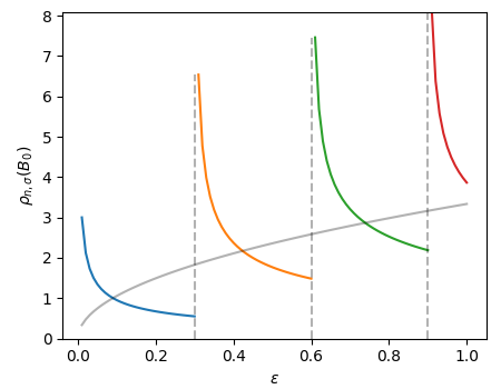
In order to understand this expression consider initially a moderate magnetic field {$B$} and the range of energies {$0\le \epsilon< \hbar\omega_c=eB/m$}. In this range {$\epsilon/\hbar \omega_c<1$} and the term {$n+(1+\sigma)/2$} can never exceed zero, otherwise the radicand becomes negative, hence {$n=0$} and {\sigma=-1$}. So we have
{$$\rho(\epsilon,B) =\frac {V}{8\pi^2 }\left( \frac {2m} {\hbar^2} \right)^{\frac 3 2} \frac {\hbar \omega_c} {\sqrt{\epsilon}}\quad\mbox{for}\, 0<\epsilon\le \hbar\omega_c$$}
In the next range {$\hbar\omega_c\le \epsilon< 2\hbar\omega_c$} there are also two contributions from {$n+(1+\sigma)/2=1$}, namely both for {$n=0,\sigma=+1$} and {$n=1,\sigma=-1$}
{$$\rho(\epsilon,B) =\frac {V}{8\pi^2 }\left( \frac {2m} {\hbar^2} \right)^{\frac 3 2} {\hbar \omega_c} \left[ \frac 1 {\sqrt\epsilon} + \frac 2 {\sqrt{\epsilon + \hbar\omega_c}}\right]\quad\mbox{for}\, \hbar\omega_c<\epsilon\le 2\hbar\omega_c$$}
and so on. This function is shown in Fig. 2.
|
(*) Notice that periodic boundary conditions may be set in the Wigner-Seitz cell, where {$-\pi/L_y\le k_y\le \pi/ L_y$}. In this case it makes sense to consider both positive and negative {$k_y$} values to yield negative and positive magnetic lengths {$x_0=\mp l^2 k_y$}. For counting purposes it is best to compare the maximum absolute value of x_0 with the crystal dimension {$L_x$} as in the text
Figure 2 Density of states (see text)
|
|
Index
Fermi energy
In order to determine the Fermi energy, that here depends on {$B$}, we calculate {$N=\int_0^{\epsilon_F(B)} \rho(\epsilon,B)d\epsilon$} as
{$$N = \frac {V\sqrt{\hbar \omega_c}}{8\pi^2 }\left( \frac {2m} {\hbar^2} \right)^{\frac 3 2}\sum_{n\sigma}\int_0^{\epsilon_F(B)} d\epsilon \left[\frac \epsilon {\hbar \omega_c}-\left(n + \frac 1 2 + \frac \sigma 2 \right)\right]^{-\frac 1 2 }$$}
The integral provides
{$$\begin{equation}N=\frac {V}{4\pi^2 }\left( \frac {2m\hbar\omega_c} {\hbar^2} \right)^{\frac 3 2}\sum_{n\sigma} \left[\frac {\epsilon_F(B)} {\hbar \omega_c}-\left(n + \frac 1 2 + \frac \sigma 2 \right)\right]^{\frac 1 2 }\end{equation}$$}
It is not possible to obtain an analytic expression for {$\epsilon_F(B)$}, so we revert to calculating the ratio of Eq. [4] to the number of occupied state in zero magnetic field, rom the usual expression {$\epsilon_F(0) = \hbar^2 (3\pi^2 N_0/V)^{\frac 2/3}/2m$}, yielding
{$$N_0=\left(\frac {2m}{\hbar^2} \right)^{\frac 3 2}\frac V {3\pi^2}\epsilon_F(0)^{\frac 3 2}$$}
In this way we obtain
{$$\frac N N_0= \frac 3 4 \left(\frac{\hbar \omega_c}{\epsilon_F(0)}\right)^{\frac 3 2} \sum_{n\sigma} \left[\frac {\epsilon_F(B)} {\hbar \omega_c}-\left(n + \frac 1 2 + \frac \sigma 2 \right)\right]^{\frac 1 2}$$}
|
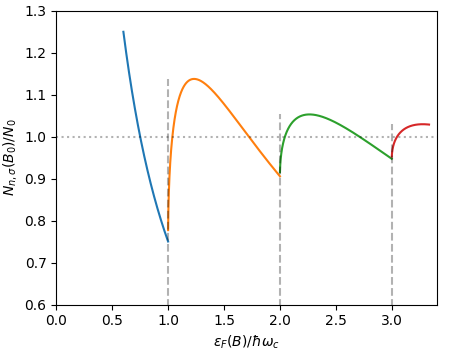 Figure 3 Ratio of total number of state for given field to the number in a B=0 Fermi gas at the same Fermi energy. The oscillation of this ration indicates indirectly the corresponding oscillation of {$\epsilon_F(B)$}. Eq. (4) is understood in the same way as Eq. (3), here versus {$\epsilon_F(0)=\epsilon_F(B)$} (in the plot in units of {$\hbar\omega_c$}). For {$0<\epsilon_F\le\hbar\omega_c$} the sum contains only the first term, {$n=0,\sigma=-1$}, for {$\hbar\omega_c<\epsilon_F\le 2\hbar\omega_c$} the sum contains two additional terms, {$n=0,\sigma=+1$} and {$n=1,\sigma=-1$}, and so on.
|
|
Index
Quantum limit
The most different state from a usual Fermi gas in zero field is attained when all electrons occupy the first Landau level, {$n=0,\sigma=1$}. This requires a very large field. Let us check this value comparing the total density with the degeneracy of the first Landau level in the quantum limit. The minimum field to enter th regime is such that {$\epsilon_F(B)=\hbar \omega_c= \frac {\hbar eB}m$} and Fig. 3 shows that this takes place for {$n =\frac3 4 n_0$}, i.e. an equivalent zero field density of {$ \frac 4 3 n$}, for which {$\epsilon_F (B) = (4/3)^{\frac 2 3}\epsilon_F(0)$}. Comparing this to the cyclotron frequency yields a field
{$$B=\frac {\hbar}{2e}(4\pi^2 n)^{\frac 2 3}$$}
The table below lists this field for a number of conductors, ranging from (compensated) intrinsic Si to Cu.High magnetic field facilities maay reach fields in the order of 100 T and perhas another order of magnitud may be obtained for short lived pulsed fields.
|